A Complete Tutorial on Self-Attention & Transformer

This article explains the Transformer architecture thoroughly, from RNN to self-attention, and then to Transformer. This is not merely a popular science article, but rather a hands-on tutorial. Readers are encouraged to ponder the questions raised throughout the article. By actively engaging with the material, you will not only gain the ability to construct a Transformer from scratch, but also develop a deep understanding of its intricate details and the rationale behind its design.

1. The Sequential Dependency Problem in RNN

RNNs struggle significantly with long-range dependencies. Here’s how RNNs are structured:

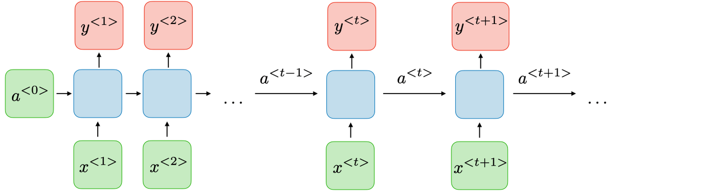
In this diagram, the input sequence is represented by $x$. The RNN first generates an initial hidden state, ${a}^{<0>}$, then performs a series of matrix multiplications with this hidden state and the corresponding tokens in the input sequence. This process generates tokens for the output sequence, denoted as $y^{<i>}$, while simultaneously updating the hidden state. Importantly, RNN is fundamentally an MLP, meaning that the blue box in the diagram isn’t a collection of separate models but a single model. Tokens from the input sequence flow sequentially through this identical MLP.

As you may have observed, the main challenge with this model stems from the hidden state update. With only one hidden state tensor, the model inevitably forgets the earlier tokens in the input sequence as the sequence grows longer. Consequently, information across the entire input sequence is treated unevenly. RNNs tend to prioritize later tokens in the sequence. This observation shares similarities with the catastrophic forgetting phenomenon encountered in online learning.

2. The Sequential Dependency Problem in LSTM

To address the limitations of RNNs, researchers developed LSTM and GRU models. Here’s a simplified representation of LSTM:

Credits

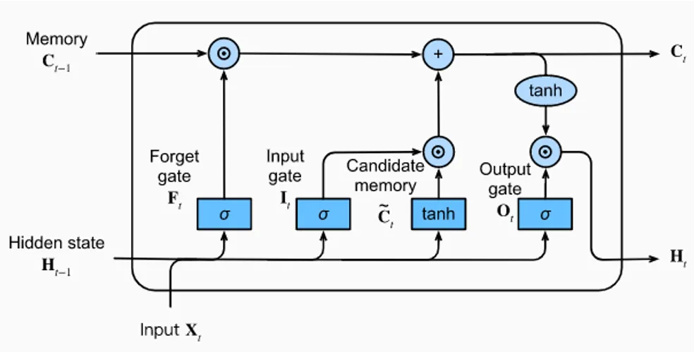
The core principle of LSTM is straightforward: retain information from previously encountered tokens. In addition to hidden states and inputs, LSTM incorporates a “backdoor” specifically designed to store past knowledge. This memory tensor, in essence, serves as another form of hidden state tensor. While this dual hidden state approach might occasionally slow down model convergence, it effectively ensures relatively long-lasting memory over extended distances. GRUs share similar ideas with LSTMs and won’t be elaborated upon here.

Although LSTMs mitigate the long-range dependency problem to some extent, the issue of information asymmetry persists. Information contained in tokens appearing earlier in the input sequence still gets compressed. LSTMs alleviate the problem but don’t fundamentally solve it. This begs the question, how would you design a model to overcome this? The answer lies in completely abandoning the sequentially dependent hidden state.

Another drawback of LSTMs lies in their limited scalability and parallelization capabilities. Accelerating RNN-based models on GPUs faces significant challenges due to the necessity of iterating through tokens one by one. The hidden state at any given time step must be derived from the hidden state at the preceding time step, highlighting the sequential dependency issue. This dependency hinders large-scale training of RNN-based models. As model parameter sizes increase, they demand substantial amounts of training data and epochs, rendering RNN models inherently slow.

3 Self-Attention: The Parallel RNN

It’s important to note that attention and self-attention are not synonymous. Attention is a broader concept encompassing self-attention, cross-attention, bi-attention, and more. This article primarily focuses on Transformer and delves into self-attention and cross-attention.

Self-attention mechanisms had been applied to various models prior to the advent of Transformer, but their effectiveness was limited. Self-attention itself has several variations, such as single-layer attention, multi-layer attention, and multi-head attention. Fundamentally, they all operate on the same principle, differing only in the number of layers or branches used. Let’s begin by examining single-layer attention.

3.1 Single-Layer Self-Attention Algorithm

The diagram below illustrates single-layer self-attention. Assuming an input sequence $x_{1,2,3}$, an embedding layer generates corresponding embeddings $a_{1,2,3}$ for each token. We then define three matrices, $Q, K, V$, as model parameters. For token embedding $a_1$, we multiply it with matrices $Q$ and $K$ to obtain vectors $q_1$ and $k_1$, respectively. Multiplying these two vectors results in an initial attention score, $at_{11}$ (often denoted as $\alpha$). It’s crucial to understand that $at_{11}$ is a scalar value, not a vector. Applying softmax to all attention scores produces normalized values, denoted as $st_{11}$. Simultaneously, $a_1$ is multiplied with matrix $V$ to yield a value vector $v_1$. Multiplying the normalized qk token with the v token gives us a qkv token, $wt_{11}$. By multiplying $q_1$ with the k vectors derived from the second and third tokens in the input sequence, we obtain $wt_{12}$ and $wt_{13}$. Summing these three tokens yields $b_1$. Repeating this process for $q_2$ and $q_3$ yields $b_2$ and $b_3$, respectively. This constitutes the core algorithm behind self-attention.

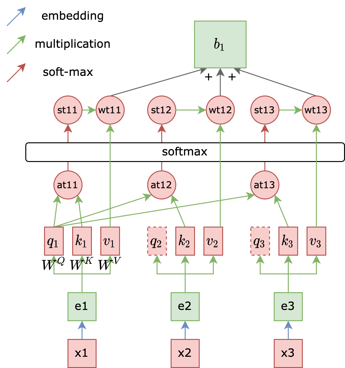
Here are some noteworthy points about the diagram:

1. The only parameters in a self-attention layer are the three matrices: ${W}^Q,{W}^K,{W}^V$.
2. The output token corresponding to each input token is essentially a weighted sum of key-value pairs from all tokens (including itself) and its own query.
3. $q, k, v$ are essentially semantic representations of the corresponding token $x$ in the latent space. Token $x$ enters the latent space as $q, k, v$ through ${W}^Q$, $W^K, W^V$.
4. The output token does not depend on the hidden state of any previous time step.

The fourth point might raise questions. Unlike RNNs, self-attention doesn’t require any hidden state that’s sequentially passed along with the tokens. This is because it employs a positional encoding method to directly modify the token embeddings, enabling the model to perceive the relative positions of tokens within the sequence. This will be explained in detail in section 4.

3.2 Matrix Representation of Self-Attention

Based on the fourth point, this algorithm can be parallelized using matrices. By concatenating the three vectors $e_{1,2,3}$ into a matrix, we get the following diagram. Since our input sequence has 3 tokens, the Inputs matrix on the left has $n = 3$. This input matrix is multiplied by three parameter matrices to obtain $Q, K, V$. Note that $Q$ and $K$ can be multiplied using ${QK}^T$ to obtain the attention score matrix. In the diagram, self-attention seems to be applied to each of the three tokens ($x_1, x_2, x_3$) separately. However, their embedding vectors can actually be concatenated for parallel processing. Similarly, concatenating $at_{11, 12, 13}$ forms a row of the attention score matrix (think about why it’s a row, not a column?). Applying row-wise softmax to this attention score matrix yields the normalized attention score matrix $A$, where each row sums to 1. The shape of matrix $A$ is $n*n$. We will delve deeper into the mathematical significance of matrix $A$ later. Finally, multiplying matrix $A$ with $V$ produces the final matrix $Z$, with a shape of $n*d_v$. This signifies that we have $n$ tokens, with each token now possessing a value of length $d_v$.

Credits

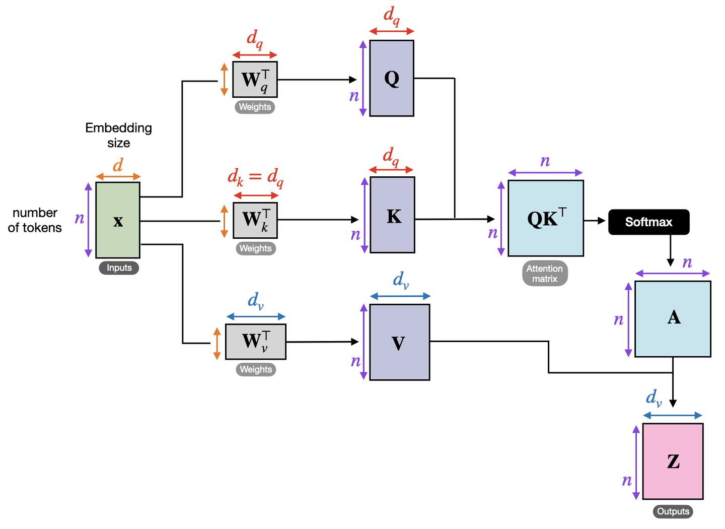
Now, let’s examine the official formula for self-attention:

Here, $Q, K, V$ represent the hidden state matrices resulting from multiplying the input matrix $X$ with three parameter matrices, respectively. $d_k$ represents the number of columns in the matrix $W_k$.

Let’s address a small detail: why divide by $\sqrt{d_k}$? Those familiar with hyperparameter tuning know that this is done to mitigate the impact of variance. If we take any column $q_i$ from matrix $Q$ and any row $k_j$ from matrix $K$, and assuming each element in $q_i$ and $k_j$ is an independently and identically distributed random variable with a mean of 0 and variance of 1, then each element in the random variable $q_i k_j^T$ (representing the attention score of token $i$ attending to token $j$) will also have a mean of 0 and a variance of 1. This is derived from the formula:

Since $q$ and $k$ are independently and identically distributed, we have:

and

\(Var(X + Y) = Var(X) + Var(Y) = \sum_m^{d_k} q_{i, m} k_{d, m} = \sum_m^{d_k} 1 = d_k\).

This means every such qk pair generates a new vector with an expected value of 0 and a variance of $d_k$, representing the attention score of token $i$ attending to token $j$. When $d_k$ is large, the variance of this vector becomes large as well. Extremely large values get pushed to the edges during the softmax layer, resulting in very small backpropagated gradients. This is where dividing by $\sqrt{d_k}$ comes in, utilizing $Var(kx) = k^2 Var(x)$ to reduce the variance from $d_k$ to 1.

3.3 The Essence of Self-Attention

Let’s delve into the essence of the official self-attention formula. Firstly, it’s essential to acknowledge that the three matrices $Q,K,V$ are essentially linear transformations of the input matrix $X$, representing $X$ semantically in the latent space. In other words, it’s possible to train the model without the matrices ${W}^Q,{W}^K,{W}^V$, but the complexity would be insufficient, impacting the model’s performance. For clarity, we’ll use $X$ to represent these three matrices. Additionally, $\frac{1}{\sqrt{d_k}}$ is used for scaling and doesn’t affect the essence, so we’ll omit it. This simplifies the official formula to:

Consider the sentence “Welcome to Starbucks.” If the embedding layer employs simple 2-hot encoding (e.g., “Welcome” is encoded as 1010), we can represent the input matrix $X$ as shown on the left side of the diagram below. Multiplying this matrix with its transpose yields a matrix that’s essentially an attention matrix, as depicted on the right side of the diagram.

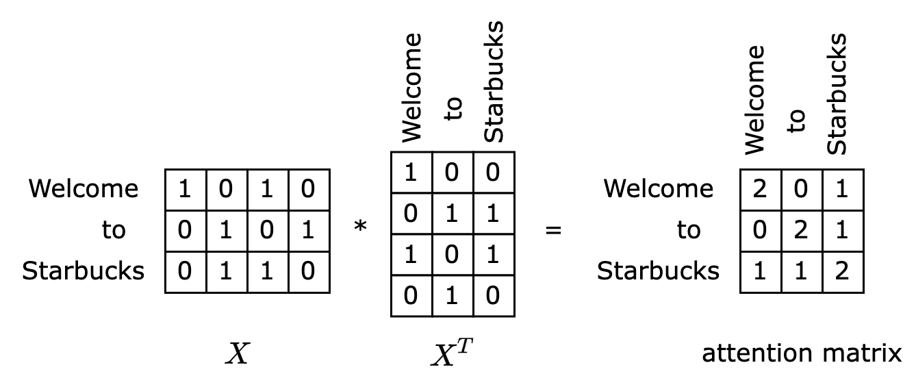
What does this attention matrix represent? Examining the first row, we see that this row essentially calculates the similarity between the token “Welcome” and all other tokens in the sentence. The essence of similarity between word vectors is attention. If token A and token B frequently co-occur, their similarity tends to be high. For instance, in the diagram, “Welcome” exhibits high similarity with itself and “Starbucks,” indicating that these two tokens should receive higher attention when inferring the token “Welcome.”

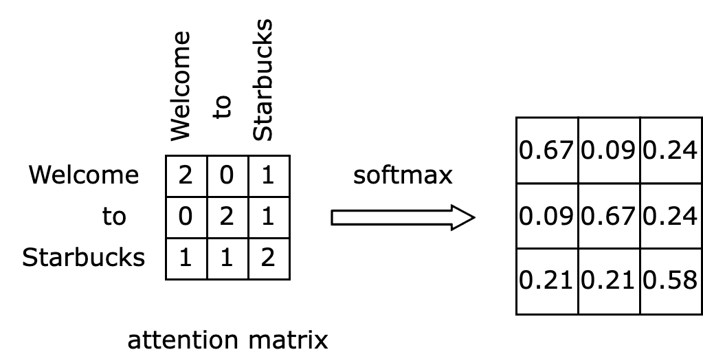
Normalizing this result using softmax gives us the normalized attention matrix shown on the right side of the diagram below. After normalization, this attention matrix becomes a coefficient matrix, ready to be multiplied with the original matrix.

The final step involves right-multiplying the normalized attention matrix $\alpha$ with the input matrix $X$, resulting in the matrix $\hat X$, as illustrated below. What does this step essentially achieve? The highlighted first row of the left matrix will be multiplied and summed with each column of the input matrix $X$ to compute each value in the first row of the output matrix. Since the first row of the $\alpha$ matrix represents the attention values of the token “Welcome” towards all tokens, the first row of the output matrix $\hat X$ becomes the attention-weighted embedding of the token “Welcome.”

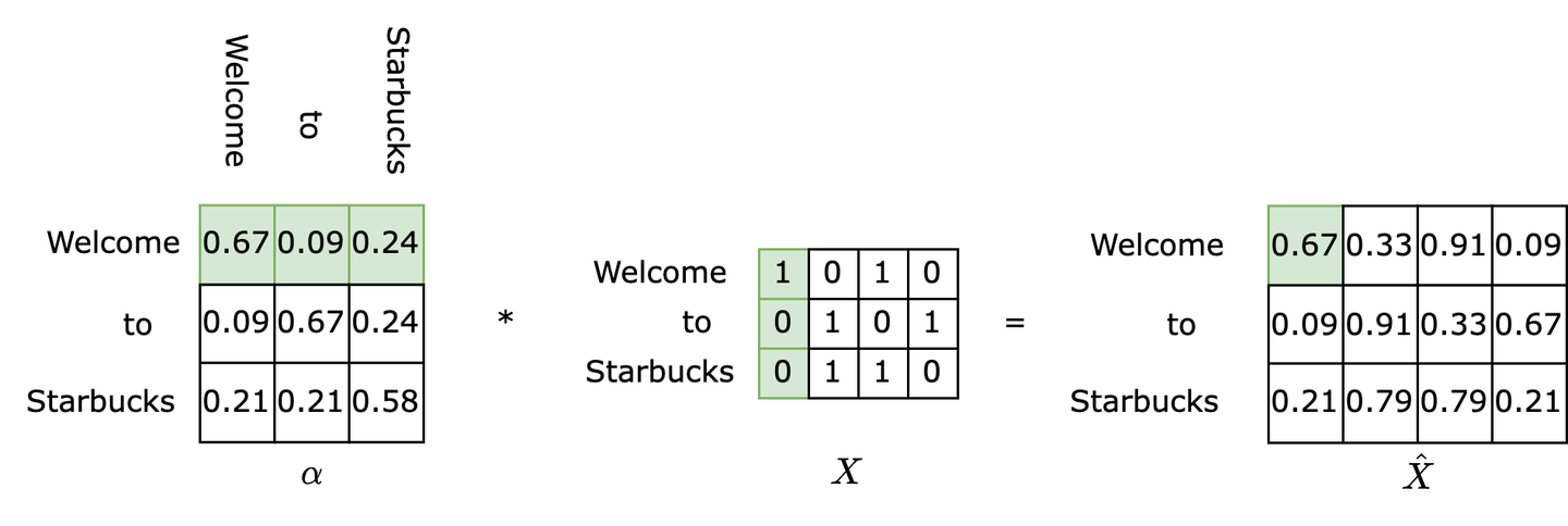
In summary, given an input matrix $\mathsf{X}$, self-attention outputs a matrix $\hat X$, which is the attention-weighted semantic representation matrix of the input matrix.

3.4 The Q, K, V Idea in Self-Attention

While the matrices $W^Q, W^K, W^V$ aren’t strictly necessary, and we know that attention weighting can be achieved using $X$ alone, the performance would be suboptimal. It’s natural to wonder how the QKV concept came about and its underlying rationale.

Why choose the names QKV? Q stands for Query, K for Key, and V for Value. In the context of databases, we aim to retrieve a corresponding Value V from the database using a Query Q. However, directly searching for V in the database using Query often yields unsatisfactory results. We desire each V to have an associated Key K that facilitates its retrieval. This Key K captures the essential characteristics of V, making it easier to locate. It’s important to note that one key corresponds to one value, implying that the number of Ks and Vs is identical.

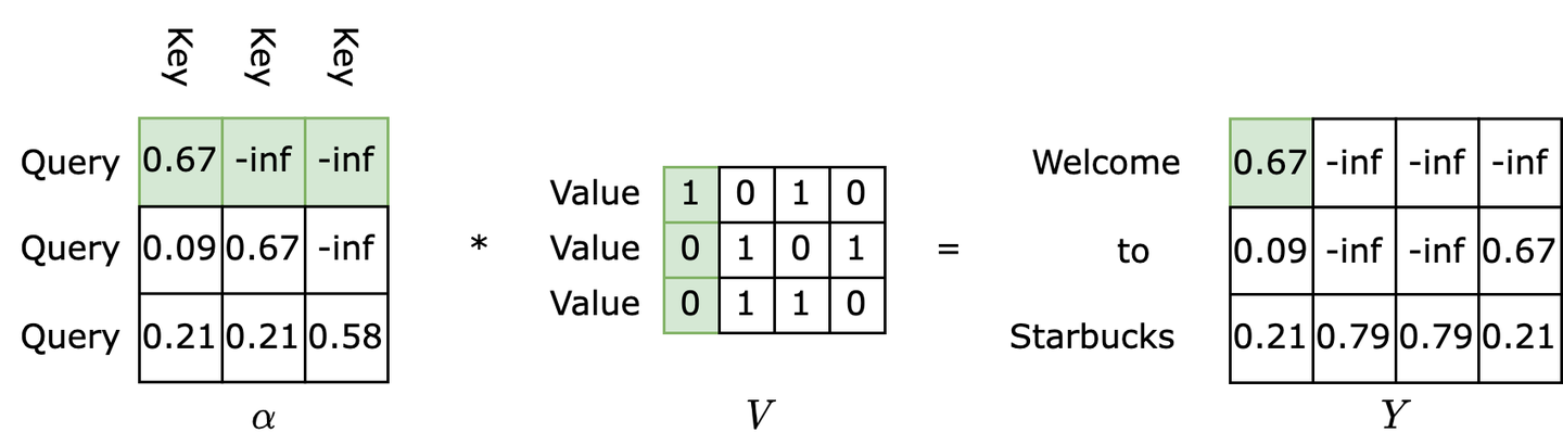
Refer to the diagram below. How are the features extracted by K obtained? Based on the attention mechanism, we need to first examine all items before accurately defining a specific item. Therefore, for each Query Q, we retrieve all Keys K (the first row of $\alpha$) as coefficients, multiply them with their corresponding Vs (the first column of V), and sum the weighted values to obtain the desired result 0.67 for this query. Through backpropagation, K gradually learns the features of V.

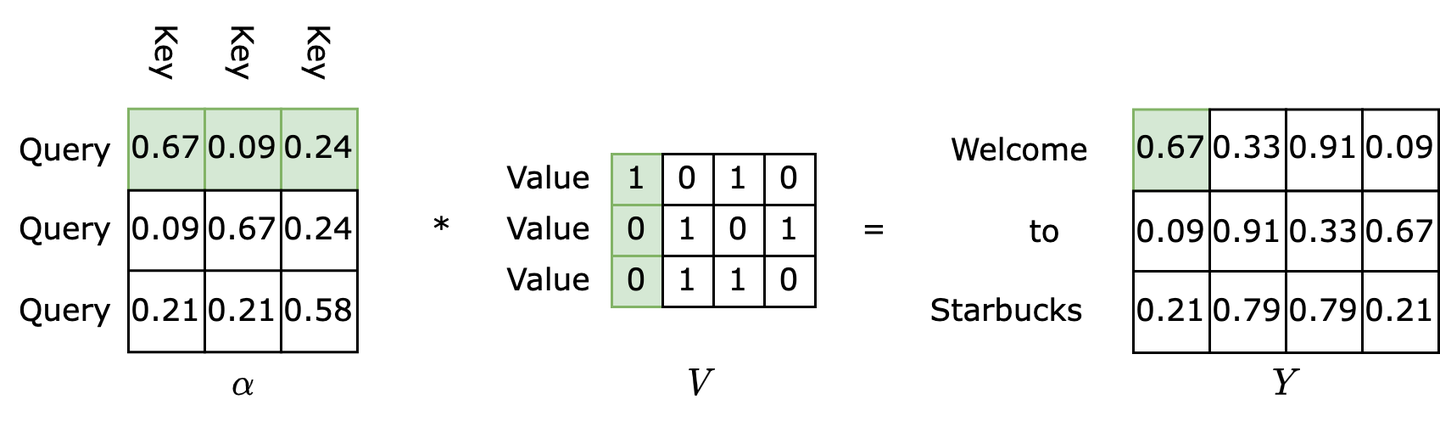
Therefore, the QKV concept in self-attention essentially functions as a database capable of integrating global semantic information. The resulting matrix Y represents the semantic matrix of the input matrix X in the latent space, with each row representing a token, having considered the contextual information.

4 Positional Encoding: Integrating Positional Information

Upon careful consideration, you’ll realize that self-attention alone, relying solely on three matrices storing semantic mappings, cannot capture positional information about tokens. The input sequence remains unaware of the order of its elements. While it’s possible to append an MLP after the output matrix Y for classification tasks, the lack of positional information hinders performance. This begs the question, how would you design an algorithm to address this issue?

The first challenge is how to integrate positional encoding into the self-attention algorithm. We could directly modify the input matrix 𝑋 or alter the self-attention algorithm itself. Modifying the input matrix is more intuitive. By ensuring that the positional embedding generated by positional encoding has the same length as the token embedding, we can directly add them to obtain a new input matrix of the same size, without requiring any modifications to the self-attention algorithm. Let’s proceed with this approach and consider how to perform the encoding.

A straightforward solution is to encode the token’s position in the sequence from 0 to 1 and incorporate it into the self-attention layer. However, this method presents a significant problem: the distance between adjacent tokens differs for sentences of varying lengths. For example, “Welcome to Starbucks” is encoded as [0, 0.5, 1] with an interval of 0.5, while “Today is a very clear day” is encoded as [0, 0.2, 0.4, 0.6, 0.8, 1] with an interval of 0.2. Such non-normalized intervals can degrade model performance, as parameters in the self-attention layer are trained in a sequence-length-agnostic manner. Introducing any sequence-length-dependent parameters can lead to parameter target alienation.

Another idea involves fixing the interval at 1 and incrementally increasing it. For instance, “Welcome to Starbucks” is encoded as [0, 1, 2], and “Today is a very clear day” is encoded as [0, 1, 2, 3, 4, 5]. While this addresses the issue of sequence-length-dependent parameters, it can result in very large parameter values for long sequences, leading to vanishing gradients.

The approach employed by Transformer is a widely used positional encoding method in applied mathematics: sinusoidal positional encoding. For a given token at position $\mathfrak{t}$ in the sequence, and embedding length $d$, the sinusoidal positional encoding is mathematically expressed as:

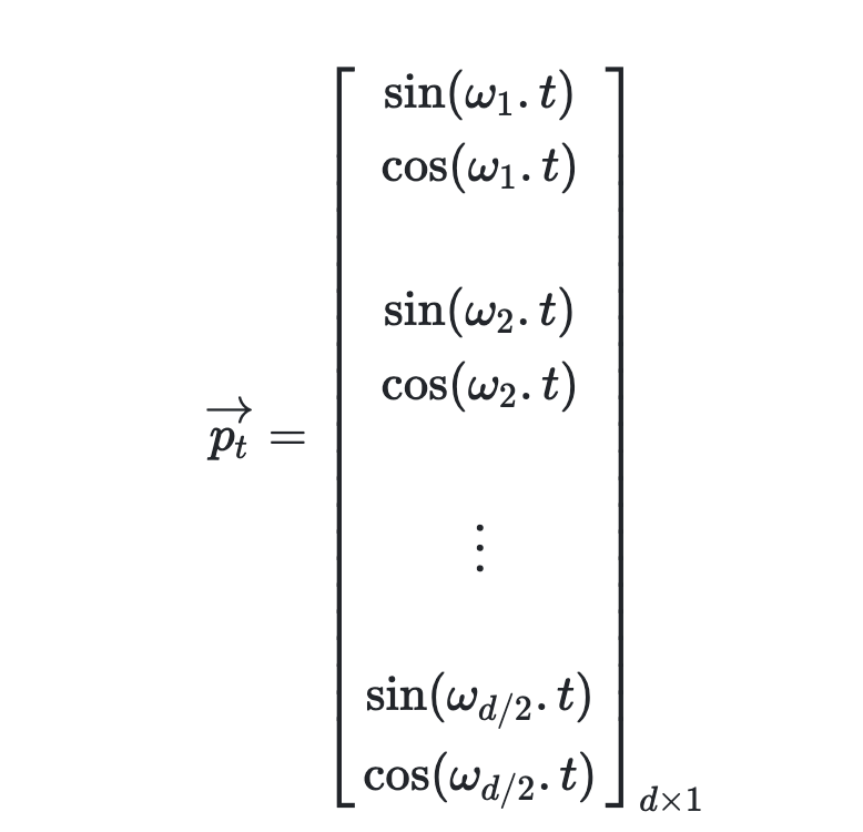
Here, $w_k=\frac{1}{10000^{2k/d}}$, $k$ is the token’s position in the sequence divided by 2, and $d$ is the embedding dimension. Notice that the length of $p_t$ is the same as the embedding length. Therefore, $p_t$ is also referred to as positional embedding and can be directly added to the semantic embedding. We can extend $\mathfrak{t}$ to the entire sequence to obtain a matrix. For example, given the input sentence “I am a Robot” with 4 tokens and embedding size $d = 4$, we can obtain the following $4 \times 4$ positional encoding matrix. Each row represents a $p_t$ from the formula above.

Credits

The first row represents the positional embedding of the token “I.” Since its position in the sequence is 0, we have $\mathrm{t} = 0$. Therefore, the first element of $p_0$ is $\sin(w_1 t)$, which is $\sin(\frac{1}{10000^{2 * 0 / 4}} * 0) = 0$. The second element is $\cos(w_1 t)$, which is $\cos(\frac{1}{10000^{20 / 4}} 0) = 1$. Following this logic, we can obtain the positional embedding for each token.

How do we interpret this method? It leverages the periodicity of the cosine function. In fact, as long as we can find multiple functions with different periods but similar characteristics (e.g., the waveform of cosine functions is the same), they can theoretically be used for positional encoding. For instance, we can employ binary positional encoding instead of sinusoidal encoding. As shown in the diagram below, assuming a sequence with 16 tokens and an embedding size of 4, we can obtain the positional embedding for each token using binary encoding:

Credits

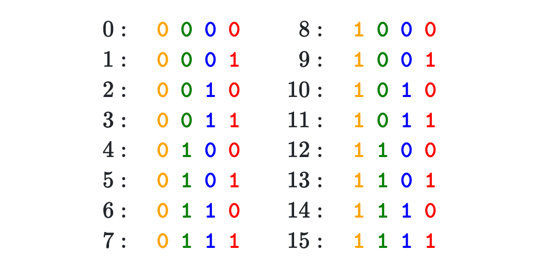
Clearly, the least significant bit (red) changes very rapidly (period of 2), while the most significant bit (yellow) changes the slowest (period of 8). This means that each positional embedding bit has a different period, preventing duplicate embeddings. Experiments have shown that this method also yields results, but not as good as sinusoidal positional encoding.

5 Transformers: Bridging the Gap in Seq2Seq

So far, we’ve established that self-attention can handle classification tasks but not seq2seq tasks. For classification, we simply add the positional embedding to $x$ to obtain the new embedding and append an MLP head after self-attention. However, seq2seq tasks often necessitate an encoder-decoder architecture. This raises the question of how to implement an encoder-decoder architecture using self-attention layers. To answer this, let’s examine how RNNs achieve this.

The diagram below illustrates the encoder-decoder architecture of an RNN. Notice that in the encoder section, the RNN performs the same operations as in classification tasks. However, at the last token, instead of connecting an MLP, the RNN passes the context vector to the decoder. The decoder is another RNN (with different parameters) that takes the context vector and the hidden vector from the previous time step as input. This RNN outputs a hidden vector and an output vector. The output vector goes through a softmax layer to obtain the probability of each token, and the token with the highest probability is selected. The hidden vector is fed back into the RNN, advancing it to the next time step. When the RNN outputs the <eos> token, the decoding process terminates, and we obtain a generated sequence, which might not necessarily have the same length as the input sequence.

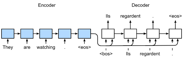
In essence, the RNN’s seq2seq solution involves obtaining a representation of the entire sentence, the context vector, in the encoder stage. This representation is then passed to the decoder, which refers to it while generating each token. Moreover, due to RNN’s sequential nature, hidden vectors remain indispensable for carrying state information.

How can we draw inspiration from RNNs to design an encoder-decoder architecture using self-attention to accomplish seq2seq tasks? Firstly, the encoder must output a representation of the processed sentence. Secondly, each token position in the decoder needs to calculate a probability to select the most likely token. However, a challenge arises: how do we pass the context vector outputted by the encoder to the decoder? In RNNs, the context vector is directly concatenated with the input embedding and fed into the RNN. If we use self-attention, can we also concatenate the context vector with the embedding and pass it to self-attention? Or should we employ an additional network for information fusion? If we use self-attention, given its three inputs, to which input should we pass the context vector?

Let’s examine the official Transformer architecture:

Credits

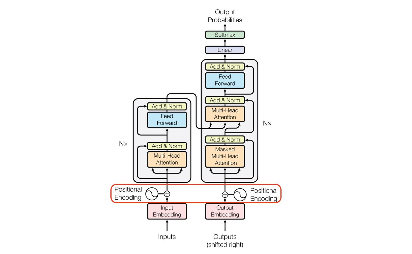
This diagram should be familiar to anyone who’s explored Transformer. The left side represents the encoder, while the right side represents the decoder. The multi-head attention layer is an enhancement over single-layer attention. The bottom left corner shows multi-head self-attention, the top right corner shows multi-head cross-attention, and the bottom right corner shows masked multi-head attention. The blue layers are FFNs (Feed Forward Layers), essentially MLPs consisting of several fully connected layers and activation functions like ReLU. Both the encoder and decoder can be stacked with multiple layers, as indicated by the $N \times$ notation in the diagram. Let’s analyze each component in detail.

5.1 Cross-Attention: Dual Tower Practice of Self-Attention

The term “cross-attention” might seem intimidating and difficult to grasp. However, if you’ve understood self-attention, cross-attention becomes quite straightforward. Why add “self” to self-attention? Looking at the Transformer architecture diagram, you’ll notice that the data input to the attention layers in the bottom left and bottom right corners both come from the same matrix, hence “self-attention.” Conversely, the data input to the attention layer in the top right corner originates from two different matrices, hence “cross-attention.”

As shown in the diagram below, we now have two input matrices, $X_1$ and $X_2$. $X_1$ provides the linear transformation $Q$, while $X_2$ provides the linear transformations $K$ and $V$. The difference between cross-attention and self-attention is marked with “new” in the diagram.

Credits

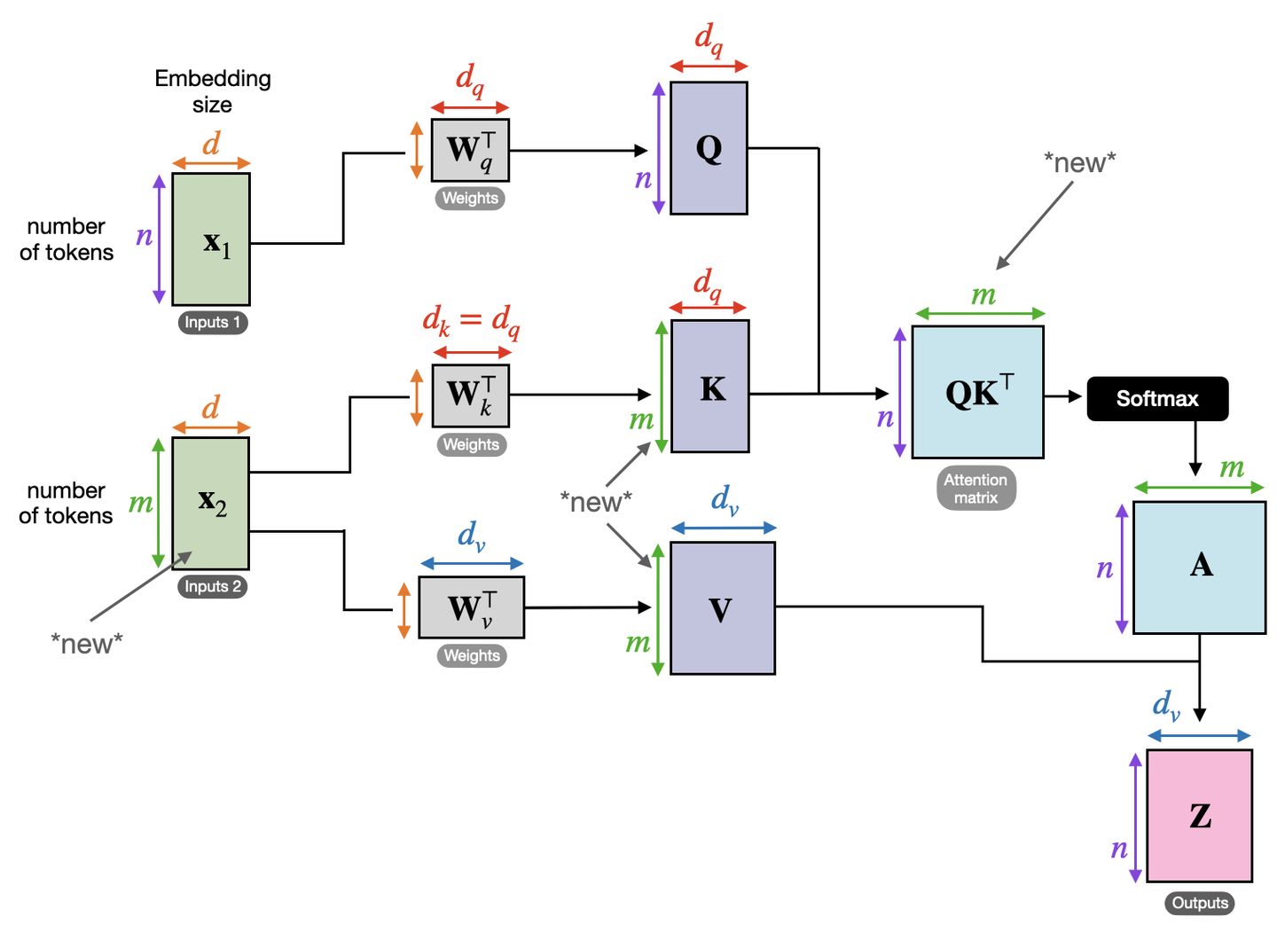
Carefully observe the resulting matrix $Z$ and you’ll see that its number of rows is the same as matrix $X_1$. Now, consider this: if you were to design the cross-attention module in the top right corner of the Transformer architecture diagram, would you use the encoder’s context vector as $X_1$ or $X_2$? Remember that the encoder’s context vector is essentially a database (V) aggregating information from the input sequence, while each input token in the decoder is essentially a query (Q), responsible for querying the database for the most similar (and therefore most important) tokens. In this light, each row in the matrix $QK^T$ in the diagram represents the attention of a decoder input token towards all tokens in the context vector. This attention matrix is called the cross-attention matrix.

5.2 Training and Prediction in Transformer Decoder

In seq2seq tasks, the Transformer encoder and decoder must be trained jointly because it’s not a classification problem, and the encoder cannot be directly connected to an MLP for training. While the flow of tokens through the encoder is relatively simple, handled by self-attention, the decoder presents some challenges. Let’s first consider this question: if you were to design how to use this decoder, could you make it output all the tokens in one go? The answer is no. Generating a sequence requires an end-of-sequence token (e.g., [EOS]) to signal termination. The generation of this end token must depend on the previously generated tokens. The decision to end a sentence relies on the sentence having fulfilled its purpose. This means the generation of the last token must be conditioned on the preceding tokens. By extension, every preceding token must be conditioned on its predecessors, all the way back to the start-of-sequence token (e.g., [SOS]). This logic mirrors human speech. While we might conceive of an entire sentence in our minds, we articulate it one word at a time, with subsequent words influenced by those preceding them. This inherent logic governs how we speak. Therefore, the decoder must still predict tokens sequentially during prediction, rather than outputting them all at once. This process of sequential token output is illustrated in the diagram below. In other words, the decoder’s prediction algorithm cannot be parallelized.

Credits

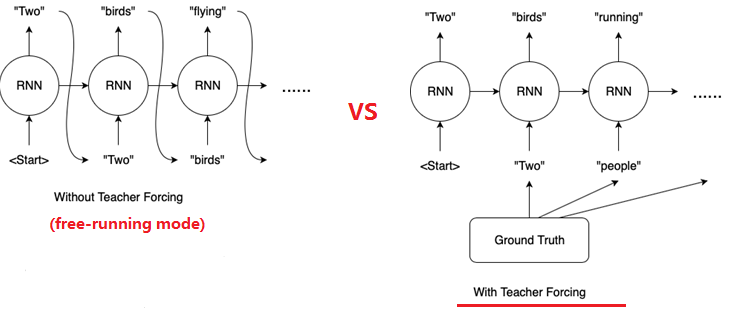
However, the decoder employs a clever training method called teacher forcing, where it learns under the guidance of a “teacher.” What does teacher forcing entail? Let’s illustrate with an example of teacher forcing in an RNN decoder. As shown in the diagram below, assume a seq2seq model receives the input “What do you see” and the correct output (label) is “Two people running.” The training process on the left is called free-running, while the one on the right is called teacher forcing. If you observe the bottom right corner of the Transformer architecture diagram, you’ll notice a “Shifted Right” operation applied to the Outputs. This involves shifting all input tokens one position to the right, corresponding to the teacher forcing method shown on the right side of the diagram below. In teacher forcing, all label tokens are shifted one position to the right, and a start-of-sequence token (e.g., <Start>) is placed at the beginning. The free-running decoder RNN receives its own output from the previous time step as input, which might be incorrect. In contrast, the teacher forcing decoder RNN receives the previous label token as input, which is guaranteed to be correct. This training method prevents the accumulation of errors, thereby improving training effectiveness.

Credits

Another advantage of teacher forcing is parallelization. The diagram above depicts an RNN. Due to the presence of a hidden vector that needs to be passed sequentially, the decoder cannot be parallelized during training. However, self-attention and cross-attention do not rely on hidden vectors for state passing. Instead, they directly encode positional information through positional embeddings during the input stage. Moreover, during training, with teacher forcing and an attention mask, we can feed the entire input and label sequences directly into the decoder (consisting of masked self-attention and cross-attention) for parallel computation and training. Therefore, by employing teacher forcing, the decoder’s training algorithm becomes parallelizable.

It’s crucial to note a subtle difference between the decoder’s prediction and training phases. During prediction, suppose we have already predicted “Welcome to.” To predict “Starbucks,” the decoder needs to see all previous tokens, “Welcome to,” not just the last token “to.” Many implementations overlook this detail and fail to stack previous tokens, resulting in poor sentence generation and a decoder that never outputs the end token. During training, due to teacher forcing and the presence of an attention mask, shifting the entire sentence to the right and feeding it into the decoder achieves the goal of attending to all previous tokens.

5.3 Masked Self-Attention: Preventing Peeking Ahead

If you think about it, simply using “Shifted Right” doesn’t fully implement teacher forcing. This is because if the attention module in the bottom right corner were unmasked self-attention, it would lead to data leakage. Let’s revisit the example from section 3.4 to see where the problem lies.

During decoding, the decoder should only have access to the tokens it has generated so far (during prediction) or the teacher tokens provided in the label up to the current time step (during training). In short, when attending to a particular token, the decoder should not be aware of any tokens appearing after it. If the decoder could attend to subsequent tokens, it would essentially be “peeking ahead” at the answers, hindering the training process.

Since self-attention relies on matrix operations, we need to employ masking to prevent this undesirable behavior. As shown in the diagram below, we can mask the upper triangular part of the attention matrix with negative infinity (-inf). By setting the attention scores of tokens that the model should not attend to as negative infinity, we prevent gradients from flowing through these positions (gradients become 0), effectively eliminating the issue of peeking ahead.

Do we need to add an attention mask to the cross-attention layer after masked self-attention? No, because the encoder has already processed the entire input sequence and possesses all the information. Therefore, the query Q from the decoder can attend to all Ks and Vs in the context vector. In other words, we allow the decoder to see all the information in the input during both training and prediction.

5.4 Multi-Head Attention: Expanding Parameter Capacity and Semantic Differentiation

The parameters learned by a single-layer attention mechanism are essentially the three matrices $W^Q, W^K, W^V$. The number of these parameters is often quite small. While this might suffice for representing basic semantics, it can become a bottleneck as semantic complexity increases. Multi-head attention addresses this limitation. Let’s see how multi-head attention in the Transformer architecture diagram differs from the single-layer attention we discussed earlier.

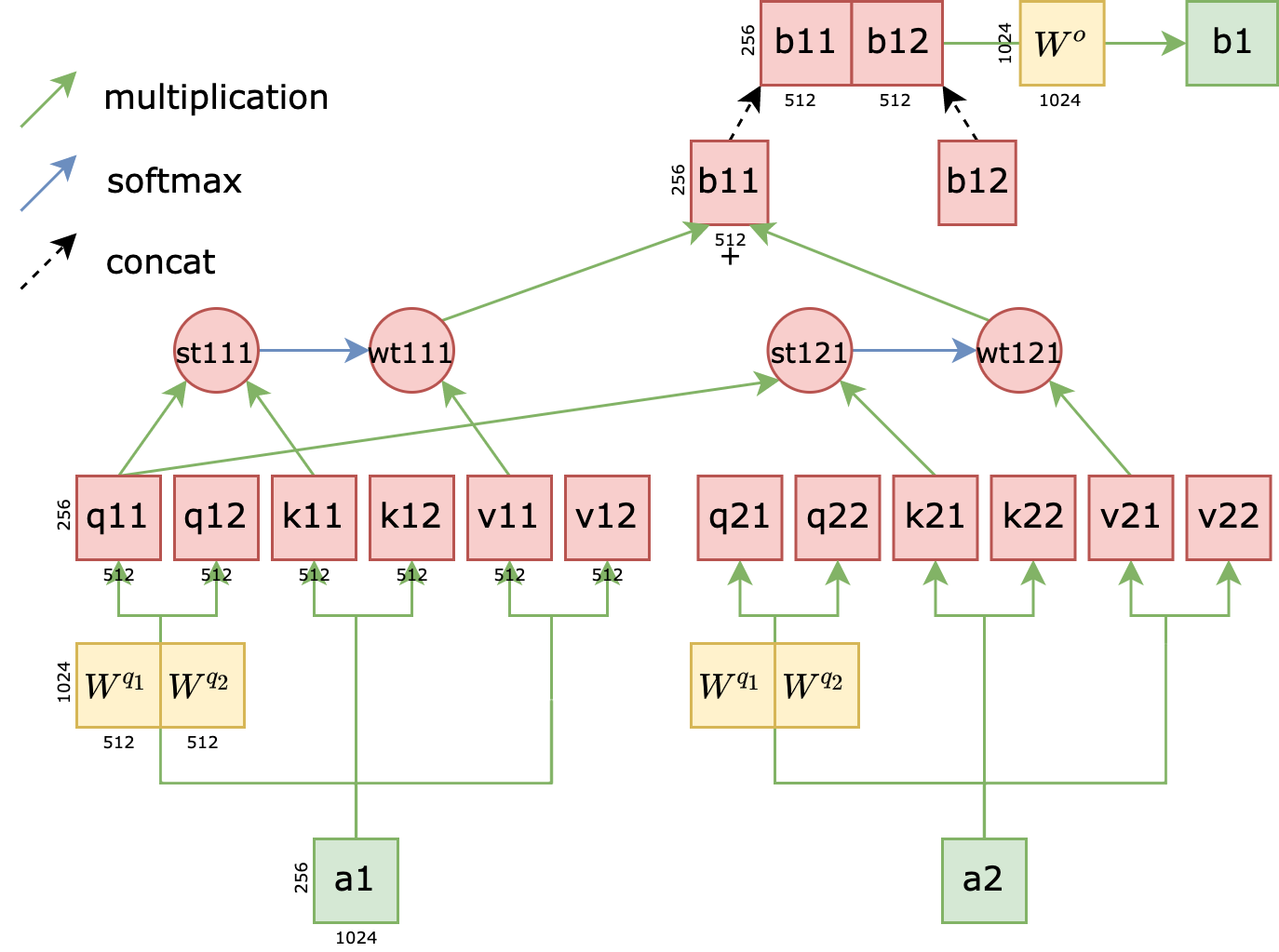
The diagram below illustrates the structure of multi-head attention. This mechanism divides the three matrices $W^Q,W^K,W^V $ into multiple smaller matrices. For instance, in a two-head attention setup, $W_Q$ is split into two smaller matrices, $W^{q_1}$ and $W^{q_2}$. Consequently, the $q$ matrix generated from $a_1$ can also be divided into two smaller matrices, $q_{11}$ and $q_{12}$, which we call attention heads. After obtaining multiple heads, the corresponding qkv heads perform single-layer attention separately, resulting in multiple outputs. For example, two heads would yield $b_{11}$ and $b_{12}$ as outputs. These outputs from different heads are then aggregated into a single output vector, $b_1$. Notice a detail in the diagram: $q_{21}$ is not used when calculating $b_1$. Think about why. Since $b_1$ represents the latent space representation of the query $a_1$, it cannot involve the query $a_2$. Refer back to section 3.4 if this isn’t clear. Once all heads have completed their calculations, an affine matrix $W_o$ is applied to aggregate information from all heads. The shapes of the matrices are indicated in the diagram. Assuming the maximum sentence length is 256 tokens and the embedding size is 1024, the shape of $a_1$ would be (256, 1024). The shapes of other matrices are also shown in the diagram.

Now that we understand the general idea, let’s explore the role of multi-head attention in more depth. Is a larger number of heads always better? Let’s examine the ablation study performed in the Transformer paper, where $h$ represents the number of heads:

Credits

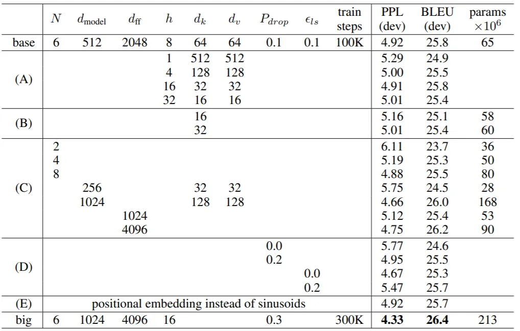
Clearly, the best performance is achieved with $h = 8$. Increasing $h$ further (to 16 or 32) doesn’t significantly improve performance, while decreasing $h$ (to 1 or 4) tends to degrade it.

Is the sole purpose of adding heads merely to increase the number of parameters? If so, we could simply enlarge the hidden size of $W^Q, W^K, W^V$. Why achieve this by adding heads?

The following diagram visualizes how different heads influence the attention matrix. This research focuses on the encoder, with 4 encoder layers (0-3), each containing 6 heads (0-5). Each row in the diagram represents an encoder layer, and each column represents a head.

Creidts

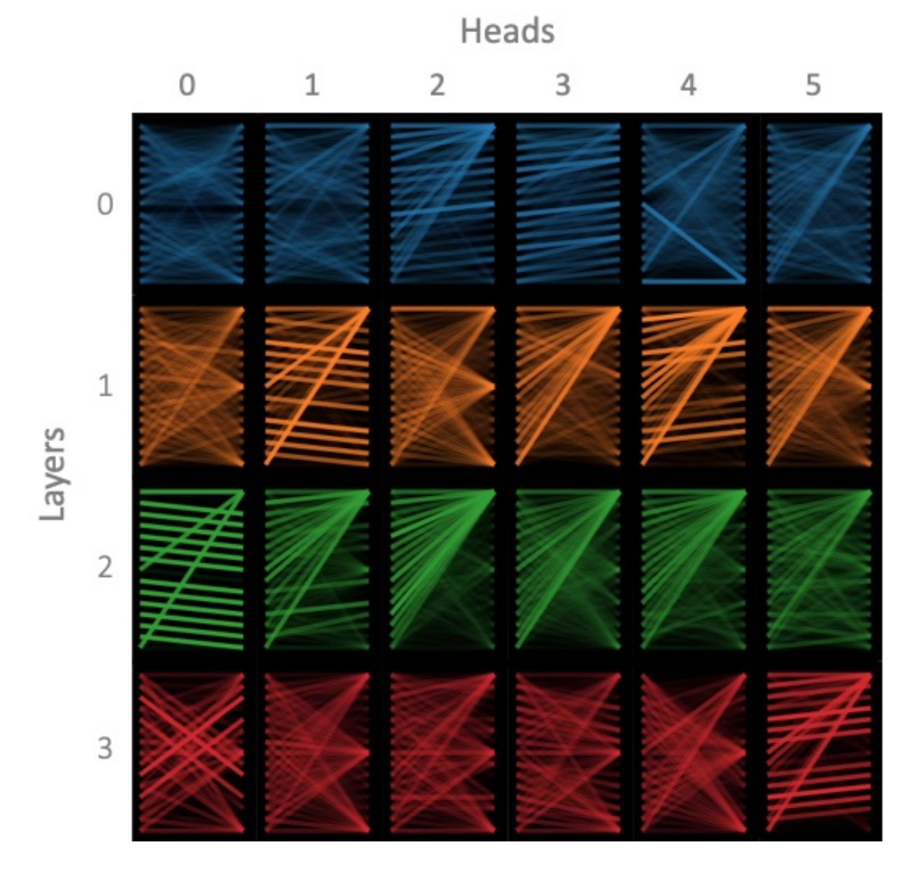
We observe that within the same layer, some heads tend to focus on similar features, while others exhibit more distinct preferences. Why do different heads select different features?

During the training of the multi-head attention mechanism, due to differences in parameter initialization, we have $q_{11} \neq q_{12}$. Similarly, we have $st_{111} \neq st_{121}$ and $b_{11} \neq b_{12}$. However, since $b_{11}$ and $b_{12}$ are concatenated, the gradient flow during backpropagation is symmetrical for these two paths. Different initialization methods lead to heads learning different feature selection capabilities.

Research has also analyzed the specific information different heads focus on. The paper “Adaptively Sparse Transformers” suggests that heads primarily focus on three aspects: grammar, context, and rare words. Grammar-focused heads effectively suppress the output of grammatically incorrect words. Context-focused heads are responsible for sentence comprehension and tend to pay more attention to nearby words. Rare word-focused heads aim to capture important keywords in the sentence. For instance, “Starbucks” is rarer than “to” and likely carries more information. Inspired by this, some research has conducted detailed ablation studies on initialization methods, demonstrating that modifying initialization can reduce layer variance and improve training effectiveness.

Let’s ponder another question: what are the significant drawbacks of using multi-layer attention (stacking multiple single-layer attention layers) instead of multi-head attention? There are substantial parallelization limitations. Multi-head attention can be easily parallelized because different heads receive the same input and perform the same computations. In contrast, due to the stacked structure of multi-layer attention, upper layers must wait for computations in lower layers to complete before proceeding, hindering parallelization. The time complexity increases linearly with the number of layers. Therefore, from a parallelization standpoint, multi-head attention is often preferred.

In summary, multi-head attention increases the parameter capacity of the attention layer, enhances the differentiation of feature extractors, and effectively improves attention performance. While more heads aren’t always better, multiple heads generally outperform a single head. Compared to multi-layer attention, multi-head attention is more conducive to parallelization.

5.5 Feed Forward Layer: Incorporating Non-Linearity

When encountering Transformer for the first time, you might be unfamiliar with the term “Feed Forward Layer” (FFN). It’s a relatively old-fashioned term. An FFN is essentially an MLP, comprising several matrices and activation functions. In the Transformer architecture diagram, FFNs appear somewhat insignificant, represented by a thin layer. However, if you carefully analyze the parameter distribution in Transformer, you’ll realize that FFNs account for more than half of the total parameters.

The FFN used in Transformer can be expressed with the following formula, where $W_1, b_1$ are the parameters of the first fully connected layer, and $W_2, b_2$ are the parameters of the second fully connected layer. A more intuitive illustration of the FFN structure is provided in the diagram below. \(W_2(\text{relu}(W_1x+b_1))+b_2\)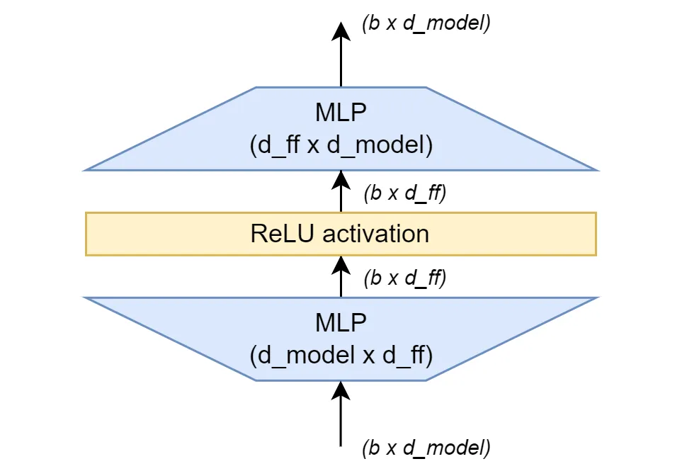

Credits

This formula allows for straightforward implementation of the FFN. Here’s a PyTorch implementation, where d_model is the embedding size (512 in Transformer) and d_ff is the hidden size of the FFN (2048 in Transformer).

class FFN(nn.Module):
    def __init__(self, d_model, d_ff):
        super(FFN, self).__init__()
        self.w_1 = nn.Linear(d_model, d_ff)
        self.w_2 = nn.Linear(d_ff, d_model)

    def forward(self, x):
        return self.w_2(F.relu(self.w_1(x)))

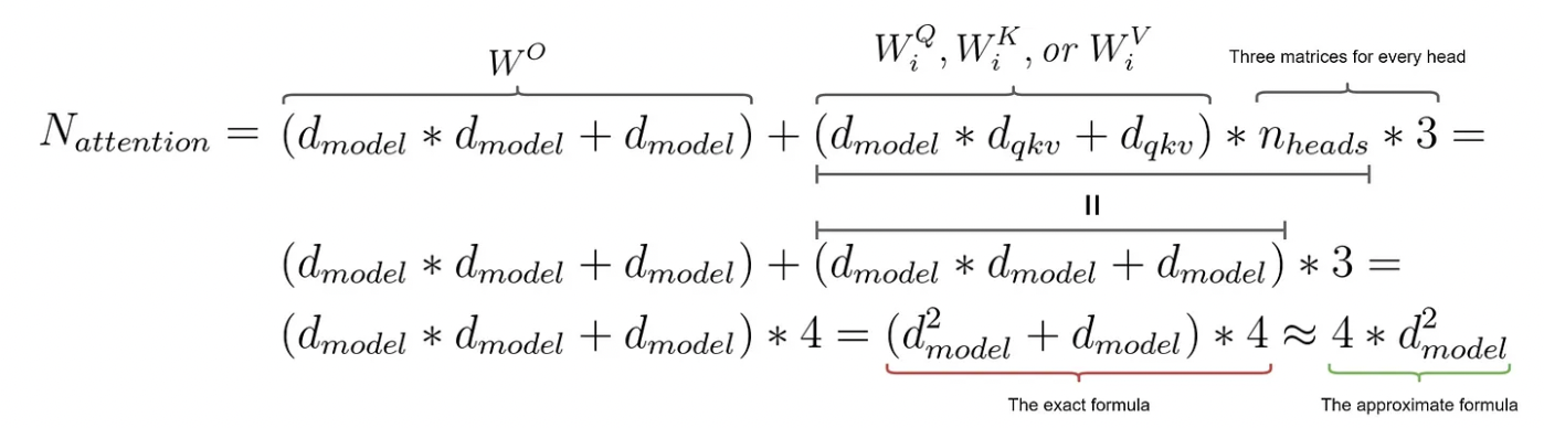
Now, let’s consider the role of this FFN layer. The embedding size dimension of the input tensor (512) is mapped to a larger hidden size dimension (2048), and then mapped back to the original embedding size (512) in the next layer. It’s evident that FFNs can introduce non-linearity into the model due to the ReLU activation function in between. Moreover, FFNs significantly increase model capacity by substantially increasing the number of parameters. Calculating the number of parameters in this FFN yields a surprisingly large number: 2∗512∗2048=2,097,152 (ignoring bias). In comparison, the article “How to Estimate the Number of Parameters in Transformer Models” states that the 8-head attention network proposed in the Transformer paper requires 1,050,624 parameters, calculated as follows:

You can verify this yourself using PyTorch:

d_model = 512
n_heads = 8
multi_head_attention = nn.MultiheadAttention(embed_dim=d_model, num_heads=n_heads)
print(count_parameters(multi_head_attention))  # 1050624
print(4 * (d_model * d_model + d_model))  # 1050624

This means that two multi-head attention layers have roughly the same number of parameters as one FFN layer. Since the Transformer architecture includes three multi-head attention layers and two FFN layers, FFNs account for over half of the total parameters.

5.6 Residual Connections and Layer Normalization

Observing the Transformer architecture diagram, you’ll notice numerous occurrences of “Add & Norm” modules, as shown below. In fact, after every computational layer, Transformer applies an “Add & Norm” module. “Add” refers to residual addition, where the input before a module is added to the output of that module to obtain a new vector. Mathematically, it’s expressed as 𝑦=𝑥+𝑓(𝑥) , where 𝑓 represents the function of the computational layer.

By the time Transformer was proposed, residual connections had become a prevalent technique for mitigating vanishing gradients, first introduced in ResNet. Whether you’re familiar with computer vision or natural language processing, you’ve likely encountered ResNet. For instance, in FFNs, the ReLU function can cause roughly half of the signals to become 0 during backpropagation, leading to significant information loss. Residual connections preserve the vector information before ReLU, effectively alleviating this issue.

In “Add & Norm,” layer normalization follows residual addition. Layer normalization, which normalizes vectors, was already widely adopted when Transformer emerged. Let’s briefly compare layer normalization with batch normalization.

As shown in the diagram below, given a three-dimensional tensor (embedding size, token number, batch size), batch normalization normalizes across a batch, while layer normalization normalizes across a sequence. For example, with a batch size of 2, suppose we input two sequences: “hello” and “machine learning.” Assume the embedding of “hello” is $[4,6,0,0]$ and the embedding of “machine learning” is $[1,2,3,3]$. Batch normalization normalizes each corresponding dimension across the batch. In other words, it normalizes each token and embedding across the two sequences. This is not ideal because tokens in the two sequences don’t necessarily correspond to each other. If we use sum-to-1 normalization, “hello” would have a normalized embedding of $[0.8,0.75,0,0]$, while “machine learning” would have a normalized embedding of $[0.2,0.25,1,1]$. This disrupts the original semantic information within the embeddings. For instance, the embedding of “hello” originally had $4<6$, but after batch normalization, it becomes $0.8>0.75$, altering the semantics.

Layer normalization, on the other hand, normalizes within each sequence, where elements naturally correspond to each other. In the example above, using layer normalization, “hello” would have a normalized embedding of $[0.4,0.6,0,0]$, while “machine learning” would have a normalized embedding of $[\frac{1}{9},\frac{2}{9},\frac{1}{3},\frac{1}{3}]$. This approach preserves the original semantics while effectively preventing gradient issues caused by excessively large values.

Credits

Conclusion

This article provided a comprehensive explanation of the various modules within the Transformer architecture. We started by discussing the limitations of RNNs, then delved into self-attention, positional encoding, the encoder-decoder architecture of Transformer, cross-attention, masked self-attention, multi-head attention, FFNs, and finally, residual connections and layer normalization.