AI for Scientific Discovery
A Warm-Up: The Cap Set Problem
热身:Cap Set 问题
Before we look at any method, let’s spend a few minutes on one concrete problem all three systems will try to solve — the cap set problem. We’ll work up to the formal statement slowly, starting from a card game you may have played. If you already know the problem from additive combinatorics, you can skim this section.
Start With the Card Game SET
从 SET 卡牌游戏说起
You may know the card game SET. Each card has four attributes — color, shape, number, shading — and each attribute takes one of three values (red/green/purple, oval/squiggle/diamond, 1/2/3, solid/striped/open). So the full deck has \(3 \times 3 \times 3 \times 3 = 81\) cards. A “SET” is three cards such that, for each of the four attributes, the three cards are either all the same or all different. Players race to spot SETs on a shared table.
Hidden inside the game is a natural puzzle:
The no-SET puzzle. Lay out a bunch of cards on the table. What’s the largest number of cards you can put down with no three of them forming a SET?
The answer is 20. You can lay 20 cards from the 81-card deck without any three forming a SET; you cannot lay 21. The constructions that achieve 20 are not obvious — they have specific structure. Our goal in the rest of this warm-up is to turn this innocent-looking card-game question into a mathematical problem you can actually attack.
Encoding the SET Rule as Math
把 SET 规则编码为数学
To reason about the no-SET puzzle we leave the cards behind and work with numbers. Label each attribute value as 0, 1, or 2. (For color, say red = 0, green = 1, purple = 2. The choice is arbitrary; what matters is that each attribute has three labels.) A card now becomes a 4-tuple of digits, e.g., \((0, 2, 1, 1)\) = “red, diamond, 2 shapes, striped”. The 81-card deck is exactly all possible such tuples. Mathematicians write this collection as \(\mathbb{F}_3^4\) — but you can read the symbol as nothing more than “4-tuples whose entries are 0, 1, or 2.”
Now look at when three cards form a SET. Pick any one attribute (one coordinate) and consider the three cards’ values there. By the SET rule, the three values are either all the same or all different. Sum the three values in each case:
- All same, e.g. \(1 + 1 + 1 = 3\). Divisible by 3.
- All different — three values \(0, 1, 2\) in some order — \(0 + 1 + 2 = 3\). Divisible by 3.
- Two same one different (a non-SET case), e.g. \(0 + 0 + 1 = 1\). Not divisible by 3.
So the SET rule, attribute by attribute, is exactly the rule “three values sum to a multiple of 3.” Stacking the four attributes back together:
Three cards \(x, y, z\) form a SET \(\iff x + y + z = (0,0,0,0)\) in \(\mathbb{F}_3^4\), where addition is taken coordinate-wise mod 3.
This is the small but important translation step. The puzzle “what’s the largest no-SET collection of cards?” has become a clean mathematical question:
What’s the largest subset of \(\mathbb{F}_3^4\) in which no three distinct elements sum to zero (mod 3)?
Cap Sets in F3n, and Why They're Hard
F3n 中的 Cap Set,以及它为什么难
There’s nothing magic about four attributes. Replace 4 with any positive integer \(n\) and you get a whole family of problems — the cap set problem:
Given \(\mathbb{F}_3^n\) (the set of \(n\)-tuples with entries in \(\{0, 1, 2\}\)), find the largest subset such that no three distinct elements sum to zero coordinate-wise mod 3. A subset with this property is called a cap set in \(\mathbb{F}_3^n\).
Small cases can be computed (or, for \(n \leq 6\), even proved exactly):
| \(n\) | 1 | 2 | 3 | 4 (SET deck) | 5 | 6 |
|---|---|---|---|---|---|---|
| Max cap set size | 2 | 4 | 9 | 20 | 45 | 112 |
For \(n \geq 7\) the exact answer is unknown; only upper and lower bounds exist. For \(n = 8\) the largest known explicit construction sits at 496 — and improving that by even one element is genuine research. FunSearch produced a construction of size 512 for \(n = 8\), which is exactly such a research-level advance.
Why is the problem so hard? The space \(\mathbb{F}_3^n\) has \(3^n\) elements, so it has \(2^{3^n}\) subsets. For \(n = 8\) that’s \(2^{6561}\), a number with roughly 1975 decimal digits. Brute-force search over subsets is hopeless. You need a construction — a clever recipe that builds a large subset while systematically avoiding any three elements that sum to zero. Such constructions are rare and typically come from deep structural insights: group theory, error-correcting codes, additive number theory.
The slow progress is telling. Between 2002 and 2023, the largest known cap set in \(\mathbb{F}_3^8\) was improved by humans only a handful of times. FunSearch’s 2023 contribution is in this slow line.
To get a visceral sense for how the constraint bites, try the simplest non-trivial case yourself. The widget below is a 3×3 grid of \(\mathbb{F}_3^2\). Click points to add them to your cap set; any three selected points whose coordinates sum to \((0, 0)\) mod 3 will be flagged with a red dashed triangle. The maximum cap set in \(\mathbb{F}_3^2\) has size 4 — try to find one. The surprise is usually how few points you need before some “wrap-around” triple snaps shut.
Why This Is the Right Yardstick
为什么它是合适的标尺
The cap set problem has three properties that make it nearly ideal as a benchmark for any LLM-driven discovery system:
- Mechanically verifiable. A few lines of Python check whether a given subset is a cap set: iterate over triples, check if any sums to zero mod 3. There is no judgment call, no need for a human or another LLM to grade the output.
- No closed form. There is no formula to derive the answer from. Every improvement is genuinely new mathematics, not a rederivation.
- Connected to deep mathematics. Cap-set sizes control the asymptotic exponent \(\omega\) of matrix multiplication via the Cohn–Umans framework. The problem is also the simplest non-trivial instance of “find dense subsets that contain no three-term arithmetic progressions” — a foundational question in additive combinatorics related to Roth’s theorem.
These three properties — easy to verify, no closed form, connected to deeper structure — are exactly what we’ll want from every benchmark in this post. FunSearch picked the cap set problem as one of its two flagship demonstrations because of them. We’ll see analogues in AlphaEvolve (the Erdős minimum-overlap problem) and TTT-Discover (the same Erdős problem, plus the autocorrelation inequality, GPU kernels, AtCoder, biology). The shape of the problem matters as much as the method.
With this concrete problem in mind, we can now look at how FunSearch, AlphaEvolve, and TTT-Discover try to solve it.
FunSearch (2023): Searching the Space of Programs
FunSearch (2023):在程序空间中搜索
The path from “LLMs as conversational assistants” to “LLMs as discovery engines” was opened by FunSearch (Romera-Paredes et al., Nature, Dec 2023). It established the template every subsequent system — including TTT-Discover — has built on: a frozen pretrained LLM proposes candidate programs, a deterministic evaluator scores them, an evolutionary outer loop selects survivors and stuffs them back into the next prompt. Understanding what FunSearch did, and where its design choices start to bind, is the cleanest entry point to the rest of this post.
The Idea: Search Over Programs, Not Outputs
核心思想:在程序而非输出上搜索
The non-obvious move in FunSearch is that the LLM is asked to produce programs that solve the problem, not answers to the problem. For a problem like “find the largest cap set in \(\mathbb{F}_3^n\),” there are at least three plausible search targets:
- The answer directly — a literal set of vectors. Hard to mutate locally, hard to characterize diversity over, and the search space scales with the answer size.
- A solver — a program that, given \(n\), returns a cap set. Compact, interpretable, runs in milliseconds, gives a clean scalar score.
- An informal proof or argument — what GPT-style chain-of-thought defaults to. Hard to verify automatically; needs an LLM-as-judge that itself becomes a noise source.
Why is a program verifiable when chain-of-thought isn’t? Both produce a final answer. The asymmetry is in how you check the answer, not in whether one exists. FunSearch’s deliverable is code: the evaluator runs it and the constructed object (a size-512 cap set, a packing of \(10^6\) items) is generated at evaluation time, then checked mechanically — a single
assertconfirms “is this a cap set?”. Chain-of-thought’s deliverable is prose, which leaves two bad options: either embed the answer literally in the text (a 512-vector list rarely survives an LLM completion intact, and parsing it back out lands you in option 1 with all its scale problems), or argue informally toward it (now verification needs to follow reasoning, which a deterministic checker cannot do — you fall back to another LLM-as-judge or a strict proof checker like Lean, the narrow path AlphaProof takes). Running code is one line of evaluator; reading prose needs parsing, trust, or both.
FunSearch picks (2). Three properties follow:
- Compactness. A 20-line Python function can generate arbitrarily large outputs (e.g., a cap set for any \(n\)). Direct-output search over strings of size proportional to the answer cannot.
- Verifiability. Run the function and compute the score. No subjective judgment, no LLM-as-judge loop, no proof checker required.
- Interpretability. A mathematician can read the resulting Python and understand what construction was discovered — sometimes well enough to generalize it into a paper-quality proof.
The “Fun” in FunSearch is function: searching in the space of functions. That naming choice telegraphs the central design commitment.
Architecture: Frozen LLM + Evolutionary Loop + Sandboxed Evaluator
架构:冻结 LLM + 演化循环 + 沙盒 evaluator
FunSearch’s loop has four components:
- Pretrained LLM. DeepMind used Codey, a PaLM 2 variant fine-tuned for code, frozen throughout. Its only role is to take a prompt of existing programs and write a new one.
- Programs database. An island-based evolutionary population. Each “island” maintains its own pool of high-scoring programs; periodic inter-island migration prevents premature convergence.
- Prompt builder. Selects \(k\) programs from the database (biased toward high scorers), formats them as in-context examples, and asks the LLM to write a better one.
- Sandboxed evaluator. Runs the candidate on the target instance, returns a scalar score. Evaluation is fast (milliseconds) and deterministic.
Crucial constraint: FunSearch evolves one function of at most around 20 lines — the “priority function” or “heuristic” that embodies the central decision the search is optimizing. Everything around it (main loop, I/O, scoring) is fixed by the human designer. This narrow target keeps per-evaluation cost tiny and lets the loop process millions of candidates in one experiment. AlphaEvolve and TTT-Discover both relax this constraint (entire files vs. single functions), and the cost structure changes accordingly.
The frozenness of the LLM is the other binding constraint, and one we will keep coming back to. FunSearch’s pretrained Codey weights are identical at iteration 1 and iteration \(10^6\). Whatever skill the system shows is amortized over all the problems Codey was ever pretrained on, plus the in-context examples assembled at runtime.
Headline Results: Cap Sets and Online Bin Packing
标志性结果:Cap Set 与在线装箱
What's online bin packing? (Click to expand)
Online bin packing: items of various sizes arrive one at a time and must be placed immediately, without knowledge of future arrivals, into bins of fixed capacity. Goal: minimize the total number of bins used. The problem is a classical operations-research staple, modeling settings from VM placement in data centers to truck loading.
Standard heuristics include First-Fit (place in the first bin with room), Best-Fit (place in the tightest bin with room), and First-Fit-Decreasing (offline; sort first). Their competitive ratios are well-studied; improving on them under realistic distributions is non-trivial because the "obvious" tweaks tend to break worst-case guarantees.
FunSearch evolved a small priority function that beats First-Fit and Best-Fit by meaningful margins on standard benchmark distributions, and is readable enough that the underlying "waste-aware" decision rule can be explained in a single sentence.
Two flagship results.
Cap set. For multiple values of \(n\), FunSearch produced larger explicit cap sets in \(\mathbb{F}_3^n\) than any previously known construction. For \(n = 8\) it produced a cap set of size 512. This is a real advance: cap-set lower bounds had been a slow-moving target in additive combinatorics, with progress measured in rare exact constructions, and FunSearch contributed one. The discovered Python function was short enough that mathematicians could read it, simplify it, and study what symmetry it was exploiting.
Online bin packing. FunSearch evolved a priority function that outperforms First-Fit and Best-Fit on multiple benchmark distributions, with a decision rule readable enough to deploy. This was the first demonstration that an LLM-driven search could discover practical algorithmic heuristics whose performance is verified by running on real workloads — not merely solve an artificial puzzle.
The two results matter for different reasons. Cap sets show the system can advance a research-level open problem. Bin packing shows it can produce practical artifacts. Both are made possible by a frozen LLM — there is no learning happening, only sampling from a fixed prior plus selection. The size of that prior and the cleverness of the prompt builder do the work. This is the design point AlphaEvolve and then TTT-Discover would push against in opposite directions.
Why FunSearch Works: Verify Is Easy, Construct Is Hard
FunSearch 为什么能成功:验证容易,构造极难
Two complementary properties make cap set the right problem for an LLM-evolutionary loop. Together they let a noisy proposer beat decades of careful human work.
Verification is cheap and exact. Given any subset \(S \subseteq \mathbb{F}_3^n\), checking whether \(S\) is a cap set takes a few lines of Python:
import itertools

def is_cap_set(S, n):
    """Return True iff no 3 elements of S sum to (0,...,0) mod 3."""
    for a, b, c in itertools.combinations(S, 3):
        if all((a[k] + b[k] + c[k]) % 3 == 0 for k in range(n)):
            return False
    return True
That’s it. No subjective judgment, no LLM-as-judge, no learned verifier. The check runs in \(O(\vert S\vert^3 \cdot n)\) time — polynomial in the size of the answer, regardless of how clever the construction was. The evaluator runs this in milliseconds on a candidate and emits a clean numerical score (typically: \(\vert S \vert\) if valid, else 0).
Construction is exponentially hard. \(\mathbb{F}_3^n\) has \(3^n\) elements and \(2^{3^n}\) subsets. For \(n = 8\) that is \(2^{6561}\) — enumeration is hopeless. Worse, naive greedy construction (“add the next compatible element”) plateaus quickly: the largest cap sets require non-local choices, where committing to a slightly worse early element opens up a much larger valid extension later. Humans have produced cap-set lower bounds slowly over decades by inventing constructions from algebraic geometry, group-theoretic symmetries, and error-correcting codes — each requiring years of domain expertise to find a single new construction worth publishing.
This is the canonical NP-style asymmetry: a valid construction is poly-time checkable, but finding one (let alone an optimal one) is exponential in the worst case. Most interesting scientific-discovery problems share this shape — theorems are easy to verify in Lean, programs are easy to run, kernels are easy to benchmark, but inventing the artifact is hard.
What FunSearch outsources. Crucially, FunSearch does not enumerate cap sets or try to “understand” them mathematically. It evolves a small priority(el) function that scores individual elements of \(\mathbb{F}_3^n\). A fixed greedy driver then builds the cap set by taking elements in priority order, rejecting any that would form a line with two already-chosen elements:
import itertools

# === The ~20-line function FunSearch EVOLVES. ===
# The published priority function for n=8 sums several modular-arithmetic
# terms; the form below sketches its structure. See Romera-Paredes et al.
# 2023, Extended Data Fig. 3, for the exact code.
def priority(el: tuple[int, ...], n: int) -> float:
    score = 0.0
    for i in range(n):
        score += LINEAR_COEFF[i][el[i]]                      # per-coordinate
    for i in range(n):
        for j in range(i + 1, n):
            score += PAIR_COEFF[i][j][el[i]][el[j]]          # pairwise
    # ... a few more terms; the coefficients embed the discovered structure
    return score

# === The FIXED driver. FunSearch does NOT evolve this. ===
def build_cap_set(n: int) -> list[tuple[int, ...]]:
    elements = list(itertools.product(range(3), repeat=n))
    elements.sort(key=lambda e: -priority(e, n))             # highest first
    chosen: list[tuple[int, ...]] = []
    for e in elements:
        # Reject if e completes a line with any pair already chosen.
        forms_line = any(
            all((a[k] + b[k] + e[k]) % 3 == 0 for k in range(n))
            for a in chosen for b in chosen if a < b
        )
        if not forms_line:
            chosen.append(e)
    return chosen
All the intellectual content lives in priority. The LLM proposes candidate priority functions; the evaluator runs build_cap_set and reports len(chosen); the evolutionary loop keeps the high-scoring ones and asks the LLM for variations. Over millions of evaluations, the search converges on priority functions whose induced greedy ordering produces unusually large cap sets — for \(n=8\), FunSearch’s discovered priority function produces a cap set of size 512.
Why this division of labor matters. Humans hit a cognitive wall when asked “how should I score an element to bias the greedy toward large constructions?” The question has millions of plausible answers, no closed form for the best one, and no obvious symmetry to exploit. A mathematician trying to write the priority function from scratch would think in terms of group orbits, linear codes, or quadratic forms — but the best priority function FunSearch finds may not match any of those: it’s a list of coefficients tuned through millions of greedy runs, each scored objectively. The LLM does not think mathematically; it samples short Python functions, each one a guess. Most are bad. A few are surprisingly good. The evaluator separates them cheaply.
The core asymmetry. Cheap to test, intractable to design. This is what lets a noisy LLM proposer plus a deterministic verifier discover what no human could write directly. AlphaEvolve and TTT-Discover both inherit this same asymmetry — on bigger problems (full code files, GPU kernels, biology pipelines) and with bigger budgets, but the underlying logic is identical.
AlphaEvolve (2025): Scaling the Template
AlphaEvolve (2025):把模板扩展上去
AlphaEvolve (DeepMind, 2025) inherits FunSearch’s shape and scales every axis of it: bigger models, longer programs, richer evaluator feedback, and the operational discipline to run all of this against problems that are economically meaningful at Google’s scale. The combination unlocks results that FunSearch’s constraints made out of reach.
What Changed: Functions to Files, One Model to Two
变了什么:函数到文件、单模型到双模型
Three architectural choices distinguish AlphaEvolve from FunSearch:
Two-tier LLM ensemble. A single run uses both Gemini 2.0 Flash (fast, cheap, generates the bulk of proposals) and Gemini 2.5 Pro (slower, smarter, used occasionally to seed harder candidates). Pure 2.5 Pro would be too expensive to run at evolutionary throughput; pure 2.0 Flash misses the deeper moves. The ensemble gets most of the throughput at Flash cost while keeping Pro’s creativity available where it counts.
Evolution at code-file granularity. Where FunSearch evolved single ≤20-line Python functions, AlphaEvolve evolves entire code files of hundreds of lines in any language. Candidates can carry non-trivial state, helper functions, even small frameworks. The trade-off is that each evaluation may take hours rather than milliseconds — but for high-value problems (kernel speedups, scheduler heuristics), that’s still worth it.
Parallel evaluators with rich feedback. Each candidate is dispatched to a parallel evaluator pool. The evaluator returns not just a scalar score but per-objective signals the next prompt can reference. The outer loop is still island-based evolution inherited from FunSearch, but populations and migration patterns are scaled up.
The cost asymmetry vs. FunSearch is the obvious downside: AlphaEvolve’s per-evaluation cost is orders of magnitude higher, so total candidates explored is orders of magnitude lower. The bet is that the richer search space (full files) and richer feedback (per-objective signals) more than compensate.
Benchmark Results: Math and Infrastructure
基准结果:数学与基础设施
What does this machinery actually produce? The headline results across math and infrastructure:
| Domain | Problem | Prior best | AlphaEvolve | Direction |
|---|---|---|---|---|
| Algorithm discovery | 4×4 complex matrix mult | 49 mults (Strassen 1969) | 48 mults | Fewer is better |
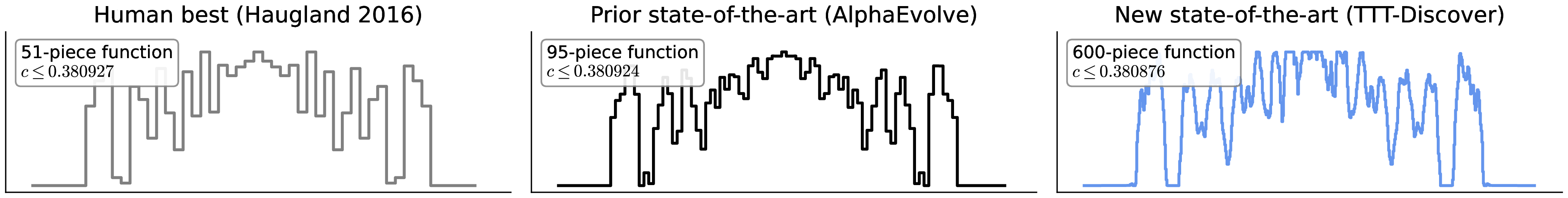
| Extremal combinatorics | Erdős minimum-overlap | 0.380927 (2016) | 0.380924 | Lower is better |
| Discrete geometry | Kissing number / packing | Various human records | Improved in several settings | Better bound |
| ML systems | Gemini training kernel | Hand-tuned baseline | ~23% speedup | Faster is better |
| Cluster scheduling | Borg scheduling heuristic | Existing production | ~0.7% compute recovered | Higher recovery |
| TPU hardware | Verilog circuit | Existing design | Reduced gate count | Fewer gates better |
What's Strassen's algorithm, and why is 48 mults a big deal? (Click to expand)
Volker Strassen showed in 1969 that the product of two 2×2 matrices can be computed with just 7 scalar multiplications (and more additions), not the obvious 8. Recursing this insight via block decomposition on n×n matrices gives runtime O(nlog2 7) ≈ O(n2.807) — the first algorithm beating the cubic O(n3) baseline. Applied once more to 4×4 = (2×2)×(2×2) the recursion gives 7×7 = 49 scalar multiplications.
That 49-mult count for 4×4 over the complex numbers stood unchallenged for 56 years, until AlphaEvolve found 48 in 2025. Earlier in 2022, AlphaTensor had already found a 47-mult algorithm for the 4×4 case — but only over the field of two elements ℤ2, not over the reals or complex numbers, so it does not apply to standard linear algebra.
The math results matter as proofs of capability: extremal problems with crisp, verifiable answers, on which AlphaEvolve unambiguously beat the human-mathematician state of the art (e.g., a 56-year-old Strassen record). The production results matter as proofs of value: deployed at Google scale, returning real compute and silicon savings. Both create non-trivial benchmarks for any successor system to target — including TTT-Discover, which directly reuses the Erdős minimum-overlap problem to claim a head-to-head win.
The Frozen-Weight Ceiling
冻结权重的天花板
Through AlphaEvolve’s entire pipeline, the LLM itself does not learn. Its weights at problem 1000 are bitwise identical to its weights at problem 1, just as FunSearch’s Codey weights were. All problem-specific behavior comes from in-context conditioning: the prompt for proposal \(N+1\) contains carefully-curated examples from \(N\). This is enormously powerful — frontier LLMs have huge implicit priors that the evolutionary loop can amplify — but it is also a ceiling.
Once the context budget is exhausted, the model cannot get better at this problem; the only remaining knob is running the loop longer and hoping a sample lands. Empirically, AlphaEvolve runs show diminishing returns after some number of generations on hard problems: the best score stops improving and the wall-clock cost per marginal advance balloons. The remedy that AlphaEvolve does not attempt is to update the model. TTT-Discover’s bet is precisely that moving the LLM’s weights themselves — modestly, RL-style, on the test problem — clears that ceiling at acceptable cost.
A Second Warm-Up: GPU Kernel Design
第二次热身:GPU Kernel 设计
TTT-Discover’s most operationally impressive results are on GPU kernels — beating hand-tuned human champions on four different chips. To appreciate why that’s a hard problem (and what TTT-Discover’s RL loop is actually searching over), we need a short tour of how GPU kernels become fast. The same warm-up-then-method pattern as the cap-set section: this part introduces the problem; the TTT-Discover section that follows shows the result.
What Is a GPU Kernel, and Why Is Making It Fast Hard?
GPU Kernel 是什么?为什么调它这么难?
A GPU kernel is a small program that runs in parallel across many threads on a GPU. A modern NVIDIA H100 has 132 streaming multiprocessors (SMs), each running thousands of threads concurrently — so a single kernel launch can have on the order of \(10^6\) thread instances in flight at once. The GPU schedules them across SMs automatically.
For matrix multiplication \(C = A \cdot B\) with \(C\) of size \(M \times N\), the simplest possible kernel — the naive kernel — assigns one thread per output element. Thread \((i, j)\) reads row \(i\) of \(A\), column \(j\) of \(B\), accumulates a \(K\)-long dot product, and writes \(C_{ij}\). Correctness is trivial; performance is terrible. Modern GPUs reach their headline TFLOPS only when the compute units are fed fast enough — and reading from HBM (high-bandwidth memory) is much slower per byte than computing on already-loaded data. The naive kernel re-reads each element of \(A\) and \(B\) many times, the SMs spend most of their cycles waiting on memory, and the achieved throughput is typically under 5% of peak.
The entire subfield of GPU kernel optimization is about closing this gap.
The Fundamental Tension: Compute vs Memory
基本张力:算力 vs 内存
Every kernel sits somewhere on a roofline:
- Memory-bound regime. Throughput is limited by how fast data arrives from HBM. To go faster, reduce bytes-moved per useful op.
- Compute-bound regime. Throughput is limited by how many FLOPs the SMs can do per cycle. To go faster, increase parallelism or use higher-throughput math units (tensor cores).
The dividing line is the kernel’s arithmetic intensity: FLOPs done per byte loaded. The crossover sits at \((\text{peak FLOPS}) \,/\, (\text{peak bandwidth})\). For an H100 with ~50 TFLOPS fp32 and ~3 TB/s memory bandwidth, that’s about 17 FLOPs/byte. Below 17, any further compute optimization is wasted; above 17, any further bandwidth optimization is wasted. Every well-tuned kernel pushes its arithmetic intensity firmly above the crossover. How depends on the operation. For matmul, the dominant tool is tiling.
Tile Size: The Key Knob
Tile Size:关键旋钮
Instead of one output element per thread, organize threads into blocks that cooperatively compute a \(T \times T\) tile of \(C\). The block first loads a strip of \(A\) (T rows, K columns) and a strip of \(B\) (K rows, T columns) into shared memory — on-chip SRAM, roughly 100× faster than HBM. The threads in the block then compute the entire \(T \times T\) tile from shared memory only, reusing each loaded element \(T\) times.
For each \(T \times T\) output tile:
- HBM bytes read: \(4 \cdot 2 T K = 8 T K\) (fp32)
- FLOPs done: \(2 T^2 K\) (one multiply + one add per \(T \times T \times K\) outer-product)
- Arithmetic intensity: \(T / 4\) FLOPs/byte
So doubling the tile size doubles the arithmetic intensity. Going from \(T = 1\) (the naive kernel) to \(T = 64\) takes you from 0.25 FLOPs/byte to 16 FLOPs/byte — right at the H100 crossover.
But \(T\) cannot grow without bound. Shared memory per block is only 48–228 KB, and each block needs \(4(T^2 + 2TK)\) bytes for the output tile and input strips. The register file and the total threads-per-block both impose further ceilings. If blocks become too big, you launch too few of them in parallel and lose occupancy — SMs sit idle for lack of work to schedule. So choosing \(T\) is a balancing act: large enough to be compute-bound, small enough to fit and to keep the SMs busy.
Try it yourself. The widget below models a simple square-tile matmul against representative GPU parameters (50 TFLOPS compute, 3 TB/s bandwidth, 48 KB shared memory per block). Slide \(T\) from 1 (the naive kernel) up through 128 (oversized) and watch the user point trace along the roofline.
The interesting band is roughly \(T \in [64, 96]\): large enough to be compute-bound, small enough to fit. Outside that band you’re leaving performance on the table. Real production kernels go much further — multi-level tiling (warp / thread / block), software pipelining, tensor-core packing, hand-tuned warp specialization, branch reduction, instruction-level scheduling — but the tile-size tradeoff is the first lever any optimizing kernel pulls.
Why TriMul Is Special (and What TTT-Discover Optimizes)
为什么 TriMul 特殊(以及 TTT-Discover 在优化什么)
The TriMul kernel is matmul with a twist: one input is restricted to upper- or lower-triangular, so half its entries are known to be zero. This pattern is ubiquitous in transformer training — the causal attention mask makes \(Q K^\top\) effectively triangular — so a fast TriMul translates directly into pretraining speedups for every causal-LM stack.
A naive kernel doesn’t know about the zeros. It loads them, multiplies by them, adds them, and wastes half the FLOPs. A specialized kernel must:
- Skip dead loads. Don’t fetch elements known to be zero — recover the lost bandwidth.
- Compress storage. Pack the triangular matrix into half the space — doubles effective bandwidth again.
- Branch-align tiles. Pick tile dimensions so each tile lies entirely above, below, or on the diagonal — never straddling, which forces warps to branch (all threads in a warp must take the same control path, so divergent branches serialize).
- Pipeline across the triangle. Reorder block iteration so warp issue rates stay high in the “thin” rows/columns near the diagonal.
These optimizations interact. The tile size that maximizes arithmetic intensity may put tile boundaries on the wrong side of the diagonal. The compressed layout that saves bandwidth may force ugly strided access patterns. Picking the best combination is what a competitive GPU engineer does over weeks of profiling.
This is the design space TTT-Discover walks. The system inherits an LLM’s prior knowledge of CUDA/Triton idioms, and uses RL to specialize a kernel for a specific TriMul shape on a specific chip. Each chip generation has different tradeoffs — H100 has tensor cores and 228 KB shared memory per block, A100 has 164 KB, AMD MI300x has wave-level instead of warp-level execution, B200 has yet another set of changes — so the optimal kernel for each chip is a different small program. The headline result you’ll see in the TTT-Discover section — beating GPUMode champions on four chip generations with one recipe — is impressive precisely because the same RL loop found a different optimum for each chip, with no human re-tuning.
TTT-Discover (2026): Training at Inference Time
TTT-Discover (2026):推理时训练
TTT-Discover keeps everything AlphaEvolve does outside the LLM — the evaluator, the prompt-building, the buffer of past programs — and changes one thing inside it: at every step, the LLM’s weights are updated by reinforcement learning, using the evaluator’s scores as reward. The rest of this section walks through what that one change buys, how it’s implemented, and how it performs on four very different problem domains.
Test-Time Training in One Paragraph
一段话讲完 Test-Time Training
Test-time training (TTT), introduced by Sun, Wang, Liu, Miller, Efros, Hardt at ICML 2020, takes a single test instance and runs a few gradient steps of a self-supervised loss on that instance before predicting. The thesis: each test instance defines its own learning problem. In 2020 the auxiliary loss was image-rotation prediction. In the 2024 sequence-modeling revival (TTT-Linear / TTT-MLP), it became an RNN inner state whose recurrence is itself a gradient step. TTT-Discover is the third act of the same idea: the “test instance” is now a scientific problem, the “auxiliary loss” is now an RL reward computed by the evaluator, and the “few gradient steps” become hundreds of RL updates on a single problem. The mechanism — train at test time, not just predict — is unchanged.
The single distinction from AlphaEvolve. AlphaEvolve: frozen LLM + evolutionary outer loop. TTT-Discover: the LLM’s weights are updated by RL using the evaluator’s scores as reward; the next batch of proposals is drawn from the updated model. Everything else is shared.
The Core Loop
核心循环
For each problem \(P\) paired with an evaluator \(E\), TTT-Discover instantiates a fresh copy of a pretrained policy \(\pi_{\theta_0}\) (the paper uses gpt-oss-120b, OpenAI’s open-source 120B-parameter model) and iterates:
init:   policy π_θ = gpt-oss-120b
        problem P with evaluator E
        rollout buffer B = ∅

for step i = 0, 1, 2, ..., N:
    # 1. PROPOSE: sample candidates from current policy
    candidates = π_θ.sample(P, batch_size=k)
    # 2. SCORE: deterministic evaluator
    rewards = E(candidates)
    B.extend(zip(candidates, rewards))
    # 3. TRAIN: RL update on the rollouts
    θ ← rl_update(θ, B)      # ← the TTT step
    # 4. KEEP BEST so far
    best = max(best, max(rewards))

return best
Single-turn rollouts, multi-step training. Each call to
π_θ.sample(...)produces a single-turn generation — the model receives a prompt (problem spec plus a few high-scoring past candidates as in-context examples) and emits one complete artifact in one shot: a Python program (math, AtCoder, biology) or a CUDA/Triton kernel (GPUMode). It does not see compiler errors, benchmark timings, or RNA-seq scores within a single rollout. The reward is computed once on the finished artifact and becomes the credit signal for the policy-gradient update on that whole output sequence. The “iteration” happens at the RL-step level — the next batch is drawn from a different policy that has absorbed the gradient signal from this batch — so the model gets progressively better at writing correct kernels first try across training steps, not across turns within one rollout. This contrasts with agentic systems like SWE-agent or Sakana’s AI CUDA Engineer, which keep the LLM frozen and instead wrap it in a multi-turn scaffold (write → compile → read error → fix → re-run → …). TTT-Discover’s bet: in domains with a fast deterministic verifier, updating the weights buys more than giving the model more turns at the same compute.
The substantive line is step 3. AlphaEvolve has steps 1, 2, 4 — and replaces step 3 with “stuff top-scoring candidates into the next prompt as in-context examples.” TTT-Discover instead does an actual RL gradient update, so that the distribution from which step 1 samples shifts toward higher-reward regions of program space as the search proceeds.
The empirical signature is visible in the reward distribution per step. The figure below, from the paper’s project page, plots the reward distribution at steps 0, 9, 24, and 49 on the GPUMode TriMul kernel competition. The whole distribution drifts upward over the course of the run — not just the maximum, but the median, the tails, the modes. The model is becoming progressively more skilled at this one problem.

(For background on GPUMode and the TriMul kernel, see the GPU kernel warm-up above.)
Reward Design, Training Recipe, and Cost
奖励设计、训练配方、成本
The 2020 TTT paper used a self-supervised auxiliary loss because vision OOD has no labels at test time. TTT-Discover’s domain is different: every problem comes with an evaluator \(E: \mathrm{candidate} \to \mathbb{R}\) — did the program compile and run? did the proof check in Lean? does the kernel produce correct output, and how fast? Those scores are labels — imperfect (high score doesn’t imply optimum), but enough to drive RL.
Two design consequences follow.
The evaluator is the bottleneck. The method’s leverage comes entirely from how informative and inexpensive \(E\) is. Each step of TTT-Discover requires evaluating a batch of candidates; the inner loop is bounded by evaluator throughput. Math conjectures get this for free (closed-form scoring); GPU kernels need a correctness checker plus a timed benchmark; competitive programming needs hidden test cases; biology needs a held-out reference. The four case studies were chosen specifically because each has a fast, reliable, densely-informative scorer.
The base model has to be capable. A weak model produces samples whose average reward is too low for the gradient to find signal. gpt-oss-120b is large enough to occasionally hit high-reward candidates from cold-start prompting — RL then amplifies that occasional hit into a reliable mode of behavior. Trying TTT-Discover on top of a 7B model would likely fail not because the method is wrong but because RL needs something to reinforce.
Practical details that matter for reproducibility:
- Backbone: gpt-oss-120b, open-source. One fresh fine-tunable copy per problem.
- Optimizer & RL objective: standard policy-gradient setup with the rollout buffer as on-policy data; details follow recent open-source RL-for-LLM recipes.
- Steps per problem: on the order of 50 RL updates (the figure shows steps 0, 9, 24, 49); each step processes a batch of new rollouts.
- Sampling at each step: thousands of candidates per step in the engineering domains; fewer when each evaluation is expensive (biology).
- Wall-clock per problem: hours to a day on commodity GPU clusters.
- Dollar cost per problem: “a few hundred dollars” per the paper — an order of magnitude below the implied AlphaEvolve per-problem cost.
The cost asymmetry comes from two places. First, gpt-oss-120b on rented GPUs is much cheaper per token than frontier-API access to a model like Gemini 2.5 Pro. Second, RL is sample-efficient compared to evolutionary search — a gradient step uses every sample in the buffer; an evolutionary step uses only the survivors. The same compute spend extracts more signal.
Math Results: Erdős & Autocorrelation
数学结果:Erdős 与自相关
Who was Erdős, and what's the minimum overlap problem? (Click to expand)
Paul Erdős (1913–1996) was a Hungarian mathematician famous for his extraordinarily prolific output — over 1500 published papers with 500+ collaborators — and for the habit of posing open problems with small cash prizes attached to their solutions. The minimum overlap problem is one of his characteristic combinatorial questions, posed in 1955.
Informally: partition the integers from 1 to 2n into two equal-sized sets A and B. Now slide one of them — consider B shifted by every integer k. The two sets B+k and A will overlap in some number of points. The minimum overlap problem asks: how small can you make the largest such overlap, by choosing A and B cleverly? Formally, define M(n) = min over partitions of max over shifts k of |A ∩ (B + k)|. Erdős conjectured that the limiting density c = limn→∞ M(n)/n is strictly bounded away from 0 and from 1/4.
The problem is hard because it's extremal: even the most evenly-spread partitions have a "bad shift" that pushes the overlap up. No closed form for c is known; every published bound corresponds to an explicit numerical construction. Improving the bound is a long-running goalpost in additive combinatorics.
For a partition of \(\{1, \dots, 2n\}\) into two equal-sized sets \(A\) and \(B\), define \(M(n) = \min_A \max_k \vert A \cap (B + k) \vert\) — the smallest possible peak overlap as you slide \(B\) over \(A\). The Erdős minimum overlap conjecture asks for the value of \(c = \lim_n M(n)/n\). Improving either bound on \(c\) has been an open problem for decades; AlphaEvolve made the first numerical progress since 2016, and TTT-Discover advances it further.
| Method | Year | Best bound on \(c\) |
|---|---|---|
| Last published human result | 2016 | 0.380927 |
| AlphaEvolve | 2025 | 0.380924 |
| TTT-Discover | 2026 | 0.380876 |
The TTT-Discover number drops the bound by about \(5 \times 10^{-5}\) below AlphaEvolve — small in absolute terms but the kind of move that takes a competition-grade specialist a year of work. Both numbers correspond to explicit constructions (partitions of \(\{1, \dots, 2n\}\) found by the search), so the result is verifiable.
The autocorrelation inequality is a sibling problem: extremal autocorrelations of indicator functions of subsets of integers. AlphaEvolve had previously pushed it; TTT-Discover takes the same problem and improves further (concrete numbers are reported alongside the Erdős result in the paper’s tables). The methodological point of the math results is not that TTT-Discover solves either conjecture — neither is solved — but that on shared problems and shared compute budgets, the test-time-training lever beats the evolutionary-search lever. That comparison is cleaner than comparing a TTT system against a different method on different problems.
Engineering: GPU Kernels and AtCoder
工程:GPU Kernel 与 AtCoder
The most operationally impressive result is on the GPUMode TriMul kernel competition: write a CUDA/Triton kernel that computes a particular triangular matrix multiplication, matching reference correctness and beating the human leaderboard on wall-clock time. The reward signal is straightforward: correctness gate × time speedup. The same TTT-Discover run was repeated on four different accelerator generations:
| Hardware | Best human (μs) | TTT-Discover (μs) | Speedup |
|---|---|---|---|
| NVIDIA A100 | 4,531 | 2,198 | 2.06× |
| AMD MI300x | 2,462 | 1,596 | 1.54× |
| NVIDIA H100 | 1,371 | 1,161 | 1.18× |
| NVIDIA B200 | 1,005 | 905 | 1.11× |
Several things to read out of this table. First, the absolute speedup is larger on older / slower chips (A100, MI300x) and shrinks on newer ones (H100, B200) — the older chips leave more room for optimization that human contestants didn’t fully exhaust, while newer chips’ theoretical peak is closer to the human submissions’ wall-clock. Second, the cross-hardware consistency — every chip beaten, including AMD — suggests the method isn’t overfitting to one vendor’s quirks. Third, the human “best” entries are the result of organized public-competition work, not casual baselines, which makes the comparison meaningful.
What's AtCoder, and how does a Heuristic Contest differ from an algorithm contest? (Click to expand)
AtCoder is a Japanese competitive programming platform, comparable in scale and prestige to Codeforces. It runs two main contest formats with very different rules.
Algorithm contests are short sessions (2–5 hours) with problems graded pass / fail — your solution either matches the expected output on every hidden test case or it does not. They reward correctness and asymptotic efficiency.
Heuristic contests (AHC) are different. They run for one to two weeks, problems are NP-hard or otherwise admit no exact polynomial-time solution, and your score is a continuous value — e.g., total cost of a schedule, number of items packed, area covered. Top submissions are the product of dozens of incremental refinements over the contest window by an experienced competitive programmer. Beating the leader by even a small margin is therefore non-trivial: it requires inventing or implementing a heuristic that the field's best didn't try.
AtCoder Heuristic Contests (AHC) are long-form competitive programming problems where the score is continuous (not pass/fail) and the goal is to maximize it — closer in flavor to “construct a good solution” than to “find the algorithm.” TTT-Discover was run on past AHC contests with the contest’s own scoring used as reward.
| Contest | Domain | Best human score | TTT-Discover score |
|---|---|---|---|
| AHC39 | Geometry | 566,997 | 567,062 |
| AHC58 | Scheduling | 847,674,723 | 848,414,228 |
The margins are small but above the best human, which on contests of this scale means the top of several hundred competitive programmers, often with multiple submissions per contestant. Same method, same model, two very different domains.
Biology: Single-Cell RNA Denoising
生物学:单细胞 RNA 去噪
Single-cell RNA-seq, PBMC, Tabula, and the classical denoisers. (Click to expand)
Single-cell RNA sequencing (scRNA-seq) measures mRNA abundance for every gene in every individual cell. The output is a (cells × genes) count matrix where entry (i, j) is approximately the number of mRNA molecules from gene j detected in cell i. Typical experiments produce 10,000 to 100,000 cells by ~20,000 genes. The matrix is brutally sparse — each cell only has a few thousand non-zero entries — and is contaminated by technical artifacts (uneven capture efficiency, amplification bias, ambient mRNA from lysed cells).
Downstream analyses (cell-type clustering, trajectory inference, marker-gene discovery) are sensitive to that noise, so denoising is a critical preprocessing step. The widely-cited classical denoisers are MAGIC (Markov affinity-based graph imputation), DCA (deep count autoencoder), and scVI (single-cell variational inference); each trains a dedicated model on the dataset.
PBMC = peripheral blood mononuclear cells, a benchmark dataset of immune cells from blood. Tabula refers to the Tabula Sapiens / Tabula Muris cell atlases — large multi-organ scRNA-seq references widely used to evaluate denoising and integration methods.
The biology case study pushes the method farthest from its comfort zone. Single-cell RNA sequencing produces sparse, noisy gene-expression counts; classical denoising methods (MAGIC, DCA, scVI) require training a domain-specific model on the dataset. TTT-Discover instead asks gpt-oss-120b to write a denoising program — a Python script that takes the raw count matrix and emits a denoised one — and uses Pearson correlation against a held-out reference as the reward signal.
| Dataset | Best human method | TTT-Discover |
|---|---|---|
| PBMC | 0.64 | 0.71 |
| Tabula | 0.64 | 0.73 |
Two-to-nine points of Pearson correlation is a meaningful margin on these benchmarks. The interesting design choice is what TTT-Discover outputs: a program, not a denoised matrix. The model is trained to be good at writing denoisers for this dataset, not at denoising itself. That inheritance from FunSearch and AlphaEvolve — programs as the unit of discovery — keeps the artifact interpretable: a biologist can read the generated Python and slot it into a real pipeline. A model that outputted a matrix directly would be hard to trust the same way.
Where This Sits, and What Comes Next
这工作的位置与下一步
Place the three milestones on a 2×2:
| Single-domain (bespoke) | Open-domain (LLM-based) | |
|---|---|---|
| Frozen at inference | Pre-2020 supervised ML | FunSearch (2023), AlphaEvolve (2025), o1/R1-style scaling |
| Updated at inference | AlphaProof’s contest-time RL (2024, narrow) | TTT-Discover (2026) |
(For reference: AlphaProof is DeepMind’s Lean-based theorem-proving system that earned a silver-medal score at IMO 2024 by running its RL training loop during the contest itself — the one prior public example of inference-time weight updates for scientific discovery, but only in the narrow Lean-proof domain.)
TTT-Discover claims the previously empty bottom-right cell: a general-purpose discovery system whose LLM is trained on whatever single problem you point it at, using off-the-shelf open weights as the cold start. The math, engineering, and biology results are the proof that this quadrant is not just theoretically interesting but currently the strongest publicly-reported configuration on the problems where direct comparisons exist.
Four threads worth flagging, two practical and two conceptual.
Practical. Does cost stay flat as problems get harder? The reported few-hundred-dollar figure is presumably averaged over problems where RL did successfully climb the reward landscape. Frontier-difficulty problems may cost much more, or fail to converge at all. Can the trained per-problem weights be reused? The paper treats each problem in isolation by design, but the specialized weights are a real asset — a “fine-tuned for kernels” model could plausibly cold-start later kernel runs faster.
Conceptual. Where does the prior come from? TTT-Discover’s RL does not invent new mathematical machinery; it amplifies structural priors already inside gpt-oss-120b’s pretraining. As problems drift further from anything in the pretraining mix, the leverage RL provides over the base model presumably shrinks. Is “test-time training” still the right framing? When you train for hundreds of GPU-hours on a single problem, the line between “test-time” and “training-time” has blurred almost beyond recognition. The deeper claim is that the unit of training has shifted from a corpus to a problem — a thesis Yu Sun’s group has been building toward since 2020, and the strongest test of which is whether the next paper extends the trajectory.