Challenges in Scaling Q-Learning
Recently, I revisited the blog by Seohong Park, “Q-learning is not yet scalable”, and would like to share some notes. In this blog, scaling is defined as whether the algorithm can solve harder problems that usually require a larger horizon, with improved data, compute, and time. There are two dimensions to scale the task difficulty: the depth and the width, which we found useful to think of in WebGym as well, when we tried to define the difficulty of a task. Seohong suggested that the depth (long-horizon) dimension is more important and harder to solve.
Why Q-Learning? The Off-Policy Advantage
为什么是 Q-Learning?离策略的优势
Before diving into the scaling challenges, it is worth understanding what makes Q-learning fundamentally different from policy gradient methods — and why researchers keep trying to scale it despite its difficulties.
Policy gradient methods (REINFORCE, PPO, etc.) are on-policy: they can only learn from trajectories generated by the current policy. If the policy changes, all previously collected data becomes stale and must be discarded or corrected via importance sampling. This is a severe constraint — it means the agent must constantly re-collect data as it improves.
Q-learning is off-policy: it learns a value function \(Q(s, a)\) that estimates the expected return of taking action \(a\) in state \(s\) and then acting optimally thereafter. The crucial property is that this Q-function can be updated from any transition \((s, a, r, s')\), regardless of which policy generated it. As Ilya Sutskever put it: off-policy means “I can learn from anyone trying to achieve any goal.”
This has profound implications. A Q-learning agent can learn from:
- Its own past experience (replay buffer), even from policies that are now outdated
- Demonstrations collected by a human or another agent
- Data generated by a completely different task, if the state-action space overlaps
In principle, this makes Q-learning far more data-efficient. In practice, however, this advantage comes with steep costs — instability, overestimation bias, and the challenges that are the subject of this post. The question is whether these costs can be overcome at scale. (See also our detailed treatment of the policy gradient family for the on-policy perspective.)
Contraction in TD Learning
TD 学习中的压缩性
For long-horizon tasks, the bias introduced by the bootstrapped TD target compounds across the bootstrapping chain. For each state-action pair, the bootstrapped target is
\[y(s, a) = r(s, a) + \gamma \max_{a'} Q_{\bar{\theta}}(s', a')\]where \(\bar{\theta}\) denotes the parameters prior to the current update. This target is biased from the true optimal value, defined as the expected discounted return under the optimal policy:
\(Q^*(s, a) = \mathbb{E}\left[\sum_{t=0}^{\infty} \gamma^t r_t \mid s_0 = s, a_0 = a\right]\)
Tabular Case
表格情形
Under a tabular setting, this bias can be systematically reduced iteration by iteration.
Define the Bellman optimality operator \(\mathcal{T}\) as:
\[(\mathcal{T}Q)(s, a) = \mathbb{E}_{s' \sim P(\cdot \mid s, a)}\left[r(s, a) + \gamma \max_{a'} Q(s', a')\right]\]Step 1: \(\mathcal{T}\) is a \(\gamma\)-contraction. For any two Q-functions \(Q\) and \(Q'\):
\[\begin{aligned} |(\mathcal{T}Q)(s,a) - (\mathcal{T}Q')(s,a)| &= \gamma \left|\mathbb{E}_{s'}\left[\max_{a'} Q(s', a') - \max_{a'} Q'(s', a')\right]\right| \\ &\leq \gamma \, \mathbb{E}_{s'}\left[\max_{a'} |Q(s', a') - Q'(s', a')|\right] \\ &\leq \gamma \|Q - Q'\|_\infty \end{aligned}\]where the first inequality uses \(\vert\max_a f(a) - \max_a g(a)\vert \leq \max_a \vert f(a) - g(a)\vert\). Taking the supremum over \((s, a)\) on the left gives
\[\lVert\mathcal{T}Q - \mathcal{T}Q'\rVert_\infty \leq \gamma \lVert Q - Q'\rVert_\infty\]By the Banach fixed point theorem, \(\mathcal{T}\) has a unique fixed point \(Q^*\) and repeated application converges:
\[\lVert\mathcal{T}^k Q - Q^*\rVert_\infty \leq \gamma^k \lVert Q - Q^*\rVert_\infty \to 0\]Step 2: Q-learning as stochastic approximation. Value iteration requires the full transition model \(P(s' \mid s, a)\) to compute the expectation in \(\mathcal{T}\). Q-learning (Watkins, 1989) removes this requirement by learning directly from experience. The agent maintains a Q-table \(Q(s, a)\) for every state-action pair, initialized arbitrarily. At each time step, the agent:
- Observes the current state \(s_t\).
- Selects an action \(a_t\) using a behavior policy (typically \(\varepsilon\)-greedy: with probability \(\varepsilon\) pick a random action, otherwise pick \(\arg\max_a Q(s_t, a)\)).
- Executes \(a_t\), observes reward \(r_t\) and next state \(s_{t+1}\).
- Updates the Q-value for the visited pair \((s_t, a_t)\):
All other entries remain unchanged: \(Q_{t+1}(s, a) = Q_t(s, a)\) for \((s, a) \neq (s_t, a_t)\). The TD error \(\delta_t\) measures how far the current estimate \(Q_t(s_t, a_t)\) is from the one-step bootstrapped target \(r_t + \gamma \max_{a'} Q_t(s_{t+1}, a')\). The learning rate \(\alpha_t \in (0, 1]\) controls the step size: larger \(\alpha\) accelerates learning but increases variance, while smaller \(\alpha\) stabilizes convergence at the cost of speed.
Why does this converge? The key insight is that the sampled TD target is an unbiased estimate of the Bellman operator applied to the current Q-function:
\[\mathbb{E}[r_t + \gamma \max_{a'} Q_t(s_{t+1}, a') \mid s_t = s, a_t = a, Q_t] = (\mathcal{T}Q_t)(s, a)\]This means each Q-learning update is, in expectation, a step of value iteration on the visited \((s, a)\) pair. The update decomposes into a contraction step plus zero-mean noise:
\[Q_{t+1}(s, a) = Q_t(s, a) + \alpha_t \left[\underbrace{(\mathcal{T}Q_t)(s, a) - Q_t(s, a)}_{\text{signal: contracts toward } Q^*} + \underbrace{\varepsilon_t}_{\text{noise}}\right]\]where
\[\varepsilon_t = \delta_t - \mathbb{E}[\delta_t \mid \mathcal{F}_t]\]is a martingale difference sequence satisfying \(\mathbb{E}[\varepsilon_t \mid \mathcal{F}_t] = 0\). Under the Robbins-Monro conditions (\(\sum_t \alpha_t = \infty\), \(\sum_t \alpha_t^2 < \infty\)) and sufficient state-action coverage, the contraction signal dominates the noise and \(Q_t \to Q^*\) almost surely.
Martingale differences and stochastic approximation. (Click to expand)
A martingale is a stochastic process whose conditional expectation of the next value, given all past information, equals the current value. Intuitively, it is a "fair game" with no drift. A sequence \(\{\varepsilon_t\}\) is a martingale difference if \(\mathbb{E}[\varepsilon_t \mid \mathcal{F}_t] = 0\), where \(\mathcal{F}_t = \sigma(s_0, a_0, r_0, \ldots, s_t, a_t, Q_t)\) is the filtration (the complete history up to step \(t\)). This means: conditioned on everything the agent has seen so far, the noise has zero expected value, i.e., it is equally likely to push the estimate up or down. Crucially, this does not require the noise to be independent across time steps; it only requires zero conditional mean.
This structure is what makes Q-learning a stochastic approximation algorithm. The general Robbins-Monro framework studies iterations of the form \(\theta_{t+1} = \theta_t + \alpha_t [h(\theta_t) + \varepsilon_t]\), where \(h(\theta^*) = 0\) defines the target fixed point. In Q-learning, \(h(Q) = \mathcal{T}Q - Q\) and \(\theta^* = Q^*\). Convergence requires:
- \(\sum_t \alpha_t = \infty\): the step sizes must be large enough in total so the iterates can travel from any initialization to \(Q^*\). If \(\sum \alpha_t < \infty\), the iterates may stall before reaching the fixed point.
- \(\sum_t \alpha_t^2 < \infty\): the step sizes must shrink fast enough so that the accumulated noise variance \(\sum \alpha_t^2 \text{Var}(\varepsilon_t)\) remains bounded. This ensures the noise averages out rather than accumulating.
A common choice satisfying both conditions is \(\alpha_t = 1/(t+1)\).
Proof that \(\varepsilon_t\) is a martingale difference. We show \(\mathbb{E}[\varepsilon_t \mid \mathcal{F}_t] = 0\).
Step 1: Compute \(\mathbb{E}[\delta_t \mid \mathcal{F}_t]\). The TD error is:
$$\delta_t = r_t + \gamma \max_{a'} Q_t(s_{t+1}, a') - Q_t(s_t, a_t)$$Since \(s_t, a_t, Q_t \in \mathcal{F}_t\), the term \(Q_t(s_t, a_t)\) is a known constant and comes out of the expectation. The only randomness is over the transition \(s_{t+1} \sim P(\cdot \mid s_t, a_t)\):
$$\mathbb{E}[\delta_t \mid \mathcal{F}_t] = \underbrace{\mathbb{E}_{s_{t+1} \sim P(\cdot \mid s_t, a_t)}\left[r(s_t, a_t) + \gamma \max_{a'} Q_t(s_{t+1}, a')\right]}_{= \, (\mathcal{T}Q_t)(s_t, a_t) \text{ by definition of } \mathcal{T}} - \; Q_t(s_t, a_t)$$The first term is exactly the Bellman operator applied to \(Q_t\), because \(\mathcal{T}\) is the expectation of the one-step bootstrapped return. Therefore:
$$\mathbb{E}[\delta_t \mid \mathcal{F}_t] = (\mathcal{T}Q_t)(s_t, a_t) - Q_t(s_t, a_t)$$Step 2: Show \(\mathbb{E}[\varepsilon_t \mid \mathcal{F}_t] = 0\). By definition, \(\varepsilon_t = \delta_t - \mathbb{E}[\delta_t \mid \mathcal{F}_t]\). Taking the conditional expectation:
$$\mathbb{E}[\varepsilon_t \mid \mathcal{F}_t] = \mathbb{E}[\delta_t \mid \mathcal{F}_t] - \mathbb{E}[\delta_t \mid \mathcal{F}_t] = 0 \quad \square$$Equivalently, \(\varepsilon_t = [r_t + \gamma \max_{a'} Q_t(s_{t+1}, a')] - (\mathcal{T}Q_t)(s_t, a_t)\) is the deviation of the sampled one-step return from its conditional mean, and the expectation of any random variable minus its own conditional expectation is zero.
Remark. This holds regardless of the behavior policy used to select \(a_t\), because by the time we condition on \(\mathcal{F}_t\), both \(s_t\) and \(a_t\) are already determined. The only source of randomness is the environment's transition \(s_{t+1} \sim P(\cdot \mid s_t, a_t)\). This is precisely why Q-learning is off-policy: the convergence proof does not depend on how actions are chosen.
Comparison with value iteration. Three important differences: (1) only one \((s, a)\) entry is updated per step, so convergence requires every state-action pair to be visited infinitely often; (2) actions must be selected by a behavior policy (e.g., \(\varepsilon\)-greedy) that balances exploration and exploitation; and (3) because Q-learning updates use \(\max_{a'}\) regardless of the behavior policy, it is an off-policy algorithm: the Q-values converge to the optimal policy even when the agent explores suboptimally.
Notice that the \(\lVert Q - Q^*\rVert_\infty\) curve in the Q-learning figure resembles a step function. This is because Q-learning updates only one \((s, a)\) entry per step, and the infinity norm is determined by the single worst-case pair. When the updated pair is not the one with the maximum error, the metric stays flat; it only jumps when the bottleneck entry itself gets updated. This staircase pattern is a direct consequence of the sparse, asynchronous nature of Q-learning. Contrast it with value iteration above, where every iteration updates all pairs simultaneously, producing a smooth exponential decay.
Function Approximation
函数近似
With a parameterized Q-function \(Q_\theta\), the tabular update \(Q(s,a) \leftarrow Q(s,a) + \alpha \delta\) becomes:
\[\theta \leftarrow \theta + \alpha \, \delta_t \, \nabla_\theta Q_\theta(s_t, a_t)\]where
\[\delta_t = r_t + \gamma \max_{a'} Q_\theta(s_{t+1}, a') - Q_\theta(s_t, a_t)\]This is called semi-gradient Q-learning because the gradient is taken only through the prediction \(Q_\theta(s_t, a_t)\), not through the bootstrapped target. In the tabular case, the semi-gradient and full gradient produce equivalent updates because each parameter controls exactly one Q-value independently; under function approximation, parameters are shared across state-action pairs, and this equivalence breaks.
Semi-gradient vs. full gradient in the tabular case. (Click to expand)
A hypothetical "full gradient" would also differentiate through the target:
$$\theta \leftarrow \theta + \alpha \, \delta_t \, \left[\nabla_\theta Q_\theta(s_t, a_t) - \gamma \nabla_\theta \max_{a'} Q_\theta(s_{t+1}, a')\right]$$In the tabular case, \(\theta \in \mathbb{R}^{|\mathcal{S}||\mathcal{A}|}\) is the Q-table. Since \(Q_\theta(s, a) = \theta_{(s,a)}\), the gradient \(\nabla_\theta Q_\theta(s, a)\) is a one-hot vector at entry \((s, a)\):
$$\left[\nabla_\theta Q_\theta(s, a)\right]_{(s',a')} = \mathbf{1}[(s',a') = (s,a)]$$Substituting, the two updates are, component-wise:
$$\text{Semi: } \theta_{(s',a')} \leftarrow \theta_{(s',a')} + \alpha\,\delta_t \cdot \mathbf{1}[(s',a') = (s_t, a_t)]$$ $$\text{Full: } \theta_{(s',a')} \leftarrow \theta_{(s',a')} + \alpha\,\delta_t \cdot \bigl\{\mathbf{1}[(s',a') = (s_t, a_t)] - \gamma\,\mathbf{1}[(s',a') = (s_{t+1}, a^*)]\bigr\}$$where \(a^* = \arg\max_{a'} Q_\theta(s_{t+1}, a')\). At the prediction entry \((s_t, a_t)\), the full gradient evaluates to \(\alpha\delta_t \cdot \{1 - \gamma \cdot \mathbf{1}[(s_t, a_t) = (s_{t+1}, a^*)]\} = \alpha\delta_t \cdot \{1 - \gamma \cdot 0\} = +\alpha\delta_t\), identical to the semi-gradient update. The \(-\gamma\) term is zero because \((s_t, a_t) \neq (s_{t+1}, a^*)\) for any non-self-loop transition. The full gradient additionally modifies a different entry \((s_{t+1}, a^*)\) by \(-\alpha\gamma\delta_t\), but since tabular parameters are decoupled, this does not interfere.
Under function approximation, \(\nabla_\theta Q_\theta(s, a)\) is no longer one-hot: updating \(\theta\) to improve \(Q_\theta(s_t, a_t)\) simultaneously changes \(Q_\theta\) at other state-action pairs. The prediction and target gradients now act on the same shared parameters, so ignoring the target gradient introduces genuine bias.
Does the semi-gradient cause Q-learning's contraction failure under FA? No — the semi-gradient introduces bias in the descent direction, but this is a separate issue from whether the operator \(\mathcal{T}\) contracts. Consider the Bellman error loss we are implicitly minimizing:
$$L(\theta) = \tfrac{1}{2}\bigl(r + \gamma \max_{a'} Q_\theta(s', a') - Q_\theta(s, a)\bigr)^2 = \tfrac{1}{2}\delta_t^2$$The true (full) gradient differentiates through both occurrences of \(\theta\):
$$\nabla_\theta L = -\delta_t \cdot \bigl[\nabla_\theta Q_\theta(s, a) - \gamma \nabla_\theta \max_{a'} Q_\theta(s', a')\bigr]$$The semi-gradient treats the target \(r + \gamma \max_{a'} Q_\theta(s', a')\) as a constant:
$$\nabla_\theta L \approx -\delta_t \cdot \nabla_\theta Q_\theta(s, a)$$This is a gradient bias: the semi-gradient is not the true gradient of \(L(\theta)\), because it ignores how \(\theta\) affects the target. It is the gradient of a different objective where the target is frozen. Note that this is distinct from the bootstrapping bias of the TD target itself: the target \(r + \gamma \max_{a'} Q_\theta(s', a')\) uses the current estimate \(Q_\theta\) rather than \(Q^*\), so it is biased regardless of whether we use semi-gradient or full gradient. The gradient bias concerns the optimization direction (how we move \(\theta\)); the bootstrapping bias concerns the target value (what we move \(\theta\) toward). Both methods compute the same (bootstrapped) TD target and apply the same operator \(\mathcal{T}\); they differ only in the descent direction. The contraction failure under FA comes from the projection \(\Pi\) onto the restricted function class, which both methods face equally.
The key question is whether Q-learning remains contractive under function approximation. It does not. As discussed above, the Bellman operator \(\mathcal{T}\) remains a \(\gamma\)-contraction, but \(\mathcal{T}Q_\theta\) generally falls outside the restricted function class, forcing a projection \(\Pi\) onto the nearest representable function. The effective update becomes
\[Q \leftarrow \Pi \mathcal{T} Q\]and
\[\lVert\Pi \mathcal{T} Q - \Pi \mathcal{T} Q'\rVert \leq \lVert\Pi\rVert \cdot \gamma \lVert Q - Q'\rVert,\]where \(\lVert\Pi\rVert\) can exceed \(1/\gamma\), destroying the contraction.
This figure illustrates two failure modes. First, the projection error floor \(\lVert\Pi Q^* - Q^*\rVert_\infty > 0\): with only 3 parameters for 10 state-action pairs, \(Q^*\) cannot be represented exactly. Second, the actual error \(\lVert Q_\theta - Q^*\rVert_\infty\) stays above even this floor. Semi-gradient Q-learning follows the TD error gradient, which is biased by bootstrapping. With the deadly triad — off-policy learning, function approximation, and bootstrapping — all present, \(\Pi \mathcal{T}\) may fail to be a contraction, causing the iterates to oscillate rather than converge.
Scaling the function class (e.g., using a language model as \(Q_\theta\)) shrinks the projection error but does not resolve the deadly triad: the composed operator \(\Pi\mathcal{T}\) can still fail to contract regardless of model capacity.
In real-world applications — robotics, game playing, large-scale decision making — the state-action space is so vast that no practical function class can represent \(\mathcal{T}Q\) exactly for all \(Q\). The projection \(\Pi\) is never the identity, and there is no guarantee that \(\Pi\mathcal{T}\) remains contractive. We should therefore not assume that Q-learning with function approximation inherits the convergence guarantees of its tabular counterpart.
Cumulative Bootstrapping Error
累积自举误差
Q-learning updates the value of state \(s\) using the estimated value of the next state \(s'\). If that estimate carries error \(\epsilon\), the update target inherits \(\gamma \epsilon\). The next state’s estimate, in turn, was built from its successor — so the error chains backward through the MDP. After \(D\) bootstrapping steps, per-state errors accumulate roughly as \(\sum_{k=0}^{D-1} \gamma^k \epsilon_k\). Longer chains mean more terms in this sum, and higher \(\gamma\) means each term decays more slowly.
For the remaining experiments, we switch to a 1-hidden-layer neural network with 64 ReLU units (257 parameters) — enough capacity to represent \(Q^*\) nearly exactly on these small MDPs. This isolates the bootstrapping dynamics from the representational limitations studied above.
Depth
深度
To see this concretely, consider chain MDPs of increasing depth: \(s_0 \to s_1 \to \cdots \to s_{D-1} \to \text{terminal}\), where only the final transition yields reward \(+1\). The shortest path is exactly \(D\) steps, and the agent must bootstrap \(Q^*\) backward through the entire chain. We fix \(\gamma = 0.9\) and use the same NN (64 ReLU units, 257 parameters) for all chains (depth 2, 8, and 32).
To see why deeper chains are harder, consider what happens step by step. In a chain of depth 5, the only grounded value is at the terminal (\(Q = 0\)). On the first Bellman backup, only \(s_4\) gets a correct target — it bootstraps from the terminal. All other states bootstrap from stale estimates (zeros), so their updates are wrong. On the second backup, \(s_3\) can now bootstrap from the corrected \(s_4\), but \(s_0\)–\(s_2\) still use incorrect values. It takes exactly \(D\) full sweeps for the correct signal to propagate from the terminal all the way back to \(s_0\).
Per-state bias
逐状态偏差
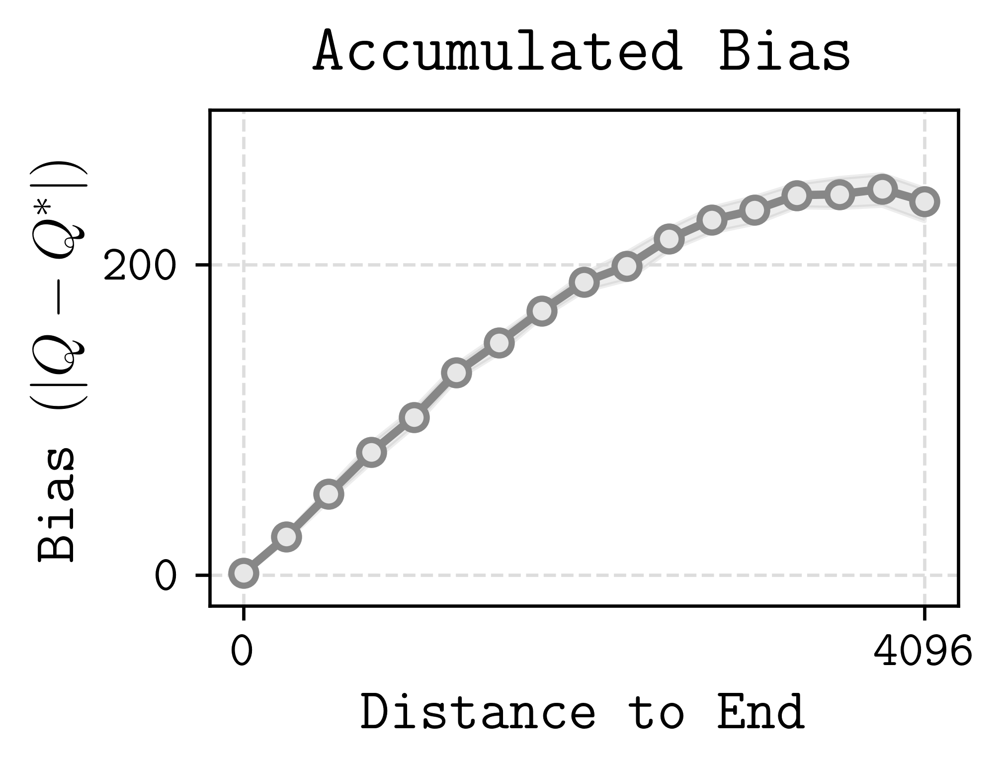
We can also look inside a single chain to see where the error lives. The figure below (from Park, 2024) plots the per-state bias against the state’s distance from the terminal. States near the terminal have small bias because bootstrapping stops there — \(Q\) is grounded at zero. States far from the terminal must propagate \(Q^*\) through many bootstrapping steps, and at each step the error in the next state’s estimate feeds into the current state’s target, compounding along the way.
Discount factor
折扣因子
This compounding effect also explains why practitioners almost never use large discount factors. The effective horizon is \(1/(1-\gamma)\): for \(\gamma = 0.99\) this is 100 steps, but for \(\gamma = 0.999\) it is 1,000 and for \(\gamma = 0.9999\) it is 10,000. Since each bootstrapping step multiplies the error by \(\gamma\), higher discount factors mean errors decay more slowly — the contraction rate weakens and the bias accumulates more severely across the chain.
Case Study: Digi-Q
案例分析:Digi-Q
The challenges above — projection error under function approximation, bootstrapping instability, and the deadly triad — are not merely theoretical. They arise directly when scaling Q-learning to real-world agentic tasks. Digi-Q (Bai, Zhou, Li, Levine & Kumar, 2025) provides a concrete case study: it trains a VLM-based Q-function for Android device control entirely from offline data, and every design choice in the paper can be read as a response to one of the failure modes discussed in this blog.
The Setup
问题设定
The agent controls a mobile device by issuing pixel-level actions (clicks, typed text) given a screenshot. Each episode is a task described in natural language (e.g., “Go to walmart.com, search for alienware area 51”). The state \(s_t\) is the interaction history up to the current screenshot; the action \(a_t\) is a string command such as “click (0.8, 0.2)”. Rewards are binary 0/1 per step, provided by an external evaluator that judges whether the task has been completed.
This is a long-horizon, large-state-space, large-action-space problem — exactly the regime where Q-learning struggles. The state space is the set of all possible screenshot histories (effectively infinite), the action space is continuous (pixel coordinates + free-form text), and episodes can span dozens of steps.
Frozen Representations and the Projection Problem
冻结表示与投影问题
The blog showed that under function approximation, the composed operator \(\Pi\mathcal{T}\) can fail to contract because \(\lVert\Pi\rVert\) may exceed \(1/\gamma\). When the function approximator is a billion-parameter VLM trained end-to-end with TD learning, this instability becomes severe: prior work (Kumar et al., 2021; Chebotar et al., 2023) found that Bellman backups on large models are “hard and unstable to train at scale.”
Digi-Q’s solution is to freeze the VLM backbone and train only a small MLP head on top of the frozen intermediate-layer representations. The Q-function becomes:
\[Q_{\theta_{\text{MLP}}}(s, a) = \text{MLP}_{\theta_{\text{MLP}}}(f_{\theta_{\text{VLM}}}(s, a))\]where \(f_{\theta_{\text{VLM}}}\) is fixed after an initial fine-tuning phase. This is a deliberate trade-off: by restricting the learnable parameters to 1% of the model, the projection \(\Pi\) onto the representable function class is more constrained (potentially larger projection error floor), but the operator \(\Pi\mathcal{T}\) behaves much more stably because the feature space does not shift during TD updates.
Digi-Q also maintains a separate state-only value function \(V_\psi\) (also an MLP on frozen VLM features) to stabilize training via double critics. The Q- and V-functions are trained with the following TD losses:
\[J_Q(\theta_{\text{MLP}}) = \mathbb{E}_{s,a,r,s' \sim \mathcal{D}}\left[(Q_{\theta_{\text{MLP}}}(f_{\theta_{\text{VLM}}}(s, a)) - r - \gamma \, V_{\bar{\psi}_{\text{MLP}}}(f_{\bar{\psi}_{\text{VLM}}}(s')))^2\right]\] \[J_V(\psi_{\text{MLP}}) = \mathbb{E}_{s \sim \mathcal{D}}\left[\mathbb{E}_{a' \sim \pi_\phi(\cdot \vert s)}\left[(V_{\psi_{\text{MLP}}}(f_{\psi_{\text{VLM}}}(s)) - Q_{\bar{\theta}_{\text{MLP}}}(f_{\bar{\theta}_{\text{VLM}}}(s, a')))^2\right]\right]\]where \(\bar{\theta}\) and \(\bar{\psi}\) are delayed target networks (exponential moving averages of \(\theta\) and \(\psi\)), following the standard trick from DQN (Mnih et al., 2013) to reduce moving-target instability. The Q-function is trained to predict the one-step bootstrapped return; the V-function is trained to match the expected Q-value under the current policy. This dual-critic setup decouples the policy evaluation (V) from the action ranking (Q), which is important for stable Best-of-N policy extraction.
Representation Fine-Tuning: Shrinking the Projection Floor
表示微调:缩小投影下界
Using off-the-shelf VLM features directly leads to a large projection error — the VLM’s internal representations are trained for general visual question answering, not for predicting the consequences of actions. Digi-Q found that without fine-tuning, the Q-function degenerates into a state-only value function \(V(s)\) that ignores the action input entirely, because the frozen features lack actionable information.
To address this, Digi-Q runs a preliminary fine-tuning phase with a binary classification objective: given a transition \((s_t, a_t, s_{t+1})\), predict whether the action caused a substantial visual change in the screen. The label is:
\[y_t = \begin{cases} 0, & d(s_t, s_{t+1}) < \epsilon \\ 1, & \text{otherwise} \end{cases}\]where \(d\) is the \(\ell_2\) image distance. This teaches the VLM to attend to which actions actually change the environment — a property the original pretraining objective never incentivized. After this phase, the VLM parameters are frozen, and the fine-tuned representations serve as the fixed feature extractor for TD learning.
In the language of our earlier discussion, this fine-tuning step shrinks the projection error \(\lVert\Pi Q^* - Q^*\rVert_\infty\) by reshaping the feature space to better capture action-relevant structure, without incurring the instability of end-to-end TD learning.
TD Learning vs. Monte Carlo
TD 学习 vs. Monte Carlo
An ablation in the paper directly tests the value of bootstrapping. Replacing TD learning with Monte Carlo (MC) regression — fitting \(Q(s, a)\) to the observed cumulative return rather than bootstrapping from \(Q(s', a')\) — drops performance from 58.0% to 37.5% on the Web Shopping benchmark.
Why does TD outperform MC here, despite the bootstrapping bias we warned about? The answer lies in variance. MC returns in this domain are extremely noisy: a single trajectory either succeeds (reward 1) or fails (reward 0), and the outcome depends on a long chain of stochastic interactions. The MC estimator is unbiased but high-variance, and this variance contaminates the Q-function when used for ranking actions. TD learning introduces bias through bootstrapping, but each update uses a one-step target with much lower variance. For the purpose of ranking actions (which is all the policy extraction needs), a slightly biased but low-variance Q-function is far more useful than an unbiased but noisy one.
This is a concrete illustration of the bias-variance tradeoff at the heart of TD learning: bootstrapping’s bias is the price of manageable variance, and in practice the tradeoff often favors TD.
Best-of-N Policy Extraction
Best-of-N 策略提取
Given a trained Q-function, the natural next step is to extract a policy. Standard approaches face their own instabilities: REINFORCE-style policy gradients suffer from a “negative gradient” term (the policy gradient multiplies the log-likelihood by the advantage, which can be negative), and advantage-weighted regression (AWR) is too conservative. Digi-Q instead uses a Best-of-N reranking approach:
- Sample \(N\) candidate actions from a behavior-cloned base policy \(\pi_\beta\).
- Score each action with the learned Q-function.
- Train the policy to imitate only the highest-scoring action (provided it has positive advantage).
Formally, the policy loss is:
\[J_\pi(\phi) = \mathbb{E}_{s_t, \, a_i \sim \pi_\beta(\cdot \vert s_t)} \left[\sum_{i=1}^{N} \delta(a_i) \sum_{h=1}^{L} \log \pi_\phi(a_i^h \vert s_t, a_i^{1:h-1})\right]\]where \(\delta(a_i) = \mathbb{1}\{a_i = \arg\max_j Q(s_t, a_j)\}\) and \(Q(s_t, a_i) - V(s_t) > 0\). This avoids the instability of policy gradients and the conservatism of AWR, while leveraging the Q-function’s ability to evaluate multiple actions at the same state — something that policy-based methods, which only see one action per state in the data, cannot do.
Performance scales monotonically with \(N\): using 16 candidate actions outperforms using 1, 4, or 8, confirming that the Q-function provides useful signal for ranking.
The Online Challenge: Distribution Shift
在线挑战:分布偏移
While Digi-Q achieves strong results in the offline setting, extending it to an online self-improvement loop — where the agent collects new data with its improved policy and retrains the Q-function — exposes a fundamental tension.
In the offline setting, the Q-function is trained on a fixed dataset \(\mathcal{D}\) collected by a behavior policy \(\pi_\beta\). The Best-of-N policy extraction produces a new policy \(\pi\) that is better than \(\pi_\beta\) but still close to it (the KL divergence is moderate, around 3.28). The Q-function only needs to be accurate for states and actions visited by \(\pi_\beta\), which is exactly what the offline data covers.
Once we enter the online loop, however, the improved policy \(\pi\) starts visiting new states that \(\pi_\beta\) never reached. The Q-function, trained only on \(\mathcal{D}\), has no reliable estimates for these out-of-distribution states. Bootstrapping from unreliable Q-values at novel states amplifies errors — precisely the compounding bootstrapping bias discussed earlier — and the critic can become arbitrarily wrong in regions of the state space that the online policy now frequents. This is a manifestation of the distribution shift problem: as the policy improves and drifts away from the data-collection policy, the Q-function’s training distribution no longer matches its evaluation distribution.
In practice, we found that this requires careful system design: periodically re-collecting data with the current policy, mixing online and offline data, and robustifying the critic against out-of-distribution inputs. The experiment iteration speed also becomes a bottleneck — each cycle of “collect data → retrain critic → extract policy” involves running the agent on real Android devices, which is orders of magnitude slower than training. These engineering challenges, rather than the core algorithmic ideas, are currently the main barrier to scaling Digi-Q’s online performance.
Takeaways
要点总结
Digi-Q illustrates how the theoretical failure modes discussed in this blog manifest in practice and how they can be mitigated with careful engineering:
| Challenge | Theory (this blog) | Digi-Q’s Response |
|---|---|---|
| Projection error \(\lVert\Pi\rVert > 1/\gamma\) | \(\Pi\mathcal{T}\) may not contract | Freeze VLM, train only MLP head |
| Large projection floor | Restricted class cannot represent \(Q^*\) | Representation fine-tuning to encode action-relevant features |
| Bootstrapping bias | Compounds over depth \(D\) | Accept bias; TD’s lower variance outperforms unbiased MC |
| Policy extraction instability | — | Best-of-N reranking avoids negative gradients |
| Online distribution shift | Q-values unreliable at novel states | Open problem; requires periodic data re-collection and critic robustification |
The result: Digi-Q’s offline Q-learning agent outperforms all prior offline methods by 21.2% on Android-in-the-Wild, and nearly matches DigiRL, which requires costly online interaction. This suggests that Q-learning can scale to complex agentic tasks — not by solving the deadly triad in general, but by carefully controlling each of its components.
References
参考文献
- Seohong Park, “Q-learning is not yet scalable”
- Nan Jiang, CS 443 Lecture 7: TD with Function Approximation, pg. 14
- Hao Bai, Yifei Zhou, Li Erran Li, Sergey Levine, Aviral Kumar, “Digi-Q: Learning VLM Q-Value Functions for Training Device-Control Agents”, ICLR 2025