Video Models and World Action Modeling

A WAM is a video model with an action head. So before unpacking the WAM designs, this section walks through the four generative-backbone ideas that the rest of the post relies on: diffusion (the loss), the diffusion transformer (DiT) and how it gets conditioned, the split between autoregressive vs diffusion video models, and flow matching (a slightly different parameterization of the same family). Two short primers — on self-attention vs cross-attention, and on where text conditioning actually enters a DiT — are slotted in where they pay off most.

WAM 就是带动作头的视频模型。所以在拆开 WAM 设计之前，这一节先把后文反复用到的四个生成式主干概念过一遍：扩散（loss）、扩散 Transformer（DiT）及其条件注入方式、视频建模中自回归 vs 扩散两种流派、以及流匹配（同一家族稍微不同的参数化）。中间还插了两段短铺垫——self vs cross attention，以及文本条件到底在 DiT 哪里——放在它们最派得上用场的位置。

The denoising diffusion probabilistic model — DDPM, Ho et al. 2020 — defines a generative process by inverting a noise-injection process. The forward process gradually corrupts data \(x_0 \sim p_{\text{data}}\) over \(T\) steps:

with \(\bar\alpha_t = \prod_{s \le t}(1-\beta_s)\). As \(t \to T\), \(x_T\) becomes pure Gaussian noise. To sample, we learn to reverse this — predict the noise component \(\epsilon\) that was added at each step:

At sampling time, we start from \(x_T \sim \mathcal{N}(0, I)\) and iteratively denoise: \(x_T \to x_{T-1} \to \ldots \to x_0\). The “diffusion” name comes from the SDE / score-matching view (Song et al. 2020): the forward process is a stochastic differential equation, the reverse is a learned score \(\nabla_x \log p_t(x)\), and the generative process is integrating that score back from noise to data. The cost is sampling latency — typically 50–1000 forward passes per sample.

去噪扩散概率模型——DDPM, Ho et al. 2020——通过反转一个加噪过程来定义生成过程。前向过程在 \(T\) 步内逐步破坏数据 \(x_0 \sim p_{\text{data}}\)：

其中 \(\bar\alpha_t = \prod_{s \le t}(1-\beta_s)\)。当 \(t \to T\) 时，\(x_T\) 变成纯高斯噪声。为了采样，我们学习反转这一过程——预测每一步加入的噪声分量 \(\epsilon\)：

采样时，从 \(x_T \sim \mathcal{N}(0, I)\) 出发迭代去噪：\(x_T \to x_{T-1} \to \ldots \to x_0\)。”扩散”这个名字来自 SDE / 分数匹配视角（Song et al. 2020）：前向过程是一个随机微分方程，反向过程是一个学到的分数函数 \(\nabla_x \log p_t(x)\)，生成就是把这个分数从噪声积分回数据。代价是采样延迟——通常每个样本需要 50–1000 次前向传播。

We can make this Markov chain concrete. The figure below traces one \(x_0 \to x_T\) trajectory using a 5×5 grid of pixels: in the forward direction, \(q\) progressively swaps blue (signal) cells for red (noise) cells until the data is gone; in the reverse direction, \(\epsilon_\theta\) is trained to undo that swap one step at a time. Toggling the two buttons swaps which formula governs the displayed direction.

我们可以把这条 Markov 链画出来。下图用一个 5×5 像素网格追踪一条 \(x_0 \to x_T\) 的轨迹：前向方向上，\(q\) 逐步把蓝色（信号）格子替换成红色（噪声）格子，直到数据消失；反向方向上，\(\epsilon_\theta\) 被训练来一步一步把这种替换还原。切换两个按钮会切换当前显示的公式。

Early diffusion models used U-Nets as the denoiser. DiT (Peebles & Xie 2022) replaced the U-Net with a transformer in order to inherit ViT’s scaling properties. The paper trains class-conditional latent DiT on ImageNet — there is no text, no cross-modal alignment, no captioning; just a 1000-way class label as the conditioning signal \(c\). Within that scope, DiT systematically explores three things: how to patchify, how to inject conditioning, and how to scale.

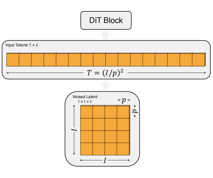
The full pipeline. A pretrained Stable-Diffusion-style VAE maps a \(256 \times 256 \times 3\) image to a \(32 \times 32 \times 4\) latent \(z = E(x)\) (downsample factor 8). DiT operates entirely in this latent space. The latent of shape \(I \times I \times C\) is patchified into a sequence of length \(T = (I/p)^2\) at hidden dim \(d\), where \(p \in \{2, 4, 8\}\) is the patch size. The token sequence is processed by \(N\) identical DiT blocks, then a final LayerNorm + linear head decodes each token back to a \(p \times p \times 2C\) tensor (noise + diagonal covariance), which is rearranged to the latent’s original spatial layout. Smaller \(p\) means more tokens, more Gflops, and — empirically — lower FID.

Encoder or decoder? Strictly, neither in the seq2seq sense. Architecturally, DiT is encoder-only (BERT / ViT-style): bidirectional self-attention, no causal mask, all latent tokens processed together, output shape = input shape. It does not autoregress. Functionally, DiT is the denoiser \(\epsilon_\theta(x_t, t, c)\) called repeatedly inside the diffusion sampling loop — input is a noised latent, output is a noise prediction. The actual encoder and decoder of the whole system are the VAE pair around DiT: the VAE encoder turns pixels into a latent before sampling starts, the VAE decoder turns the final cleaned latent back into pixels. DiT sits between them and is neither — it’s the iteratively-applied refiner.

早期扩散模型用 U-Net 作为去噪网络。DiT（Peebles & Xie 2022）把 U-Net 换成了 Transformer，目的是继承 ViT 的 scaling 性质。论文训练的是类别条件、潜空间的 DiT，数据集是 ImageNet——没有文本、没有跨模态对齐、没有 captioning，条件 \(c\) 就是一个 1000 类的标签。在这个范围内，DiT 系统地探索了三件事：怎么 patchify、怎么注入条件、怎么 scale。

完整流水线。 一个预训练的 Stable Diffusion 系列 VAE 把 \(256 \times 256 \times 3\) 的图像映射成 \(32 \times 32 \times 4\) 的潜变量 \(z = E(x)\)（下采样 8 倍）。DiT 全程在这个潜空间里操作。形状 \(I \times I \times C\) 的潜变量被 patchify 成长度为 \(T = (I/p)^2\)、隐藏维度为 \(d\) 的 token 序列，patch size \(p \in \{2, 4, 8\}\)。token 序列进入 \(N\) 个相同的 DiT block 处理，最后一个 LayerNorm + 线性头把每个 token 解码回形状 \(p \times p \times 2C\) 的张量（噪声 + 对角协方差），再 rearrange 回潜变量原本的空间布局。\(p\) 越小，token 越多、Gflops 越大，经验上 FID 也越低。

算 encoder 还是 decoder？ 严格说，seq2seq 意义上两者都不是。架构上，DiT 是 encoder-only 的（BERT / ViT 风格）：双向 self-attention、没有 causal mask、所有 latent token 一起处理、输出形状 = 输入形状，不做自回归。功能上，DiT 是扩散采样循环里反复调用的去噪网络 \(\epsilon_\theta(x_t, t, c)\)——输入带噪 latent，输出噪声预测。整个系统真正的 encoder 和 decoder 是 DiT 外面那对 VAE：VAE encoder 在采样前把像素压成 latent，VAE decoder 在最后把去干净的 latent 解回像素。DiT 夹在中间，两者都不是——它是一个被反复调用的 refiner。

Figure 4 of the paper visualizes the patchify operation in concrete shape terms.

论文 Figure 4 用具体形状把 patchify 这一步可视化了。

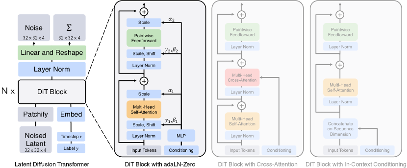
Four block designs for injecting conditioning. Once the image is a sequence of tokens, the question is how to feed the network the noise level \(t\) and the class label \(c\). The DiT paper explicitly considers four variants — these are exactly the panels on the right of Figure 3:

1. In-context conditioning. Append the embeddings of \(t\) and \(c\) as two extra tokens to the input sequence (like ViT’s [CLS] token). Let standard self-attention mix them with the image tokens; remove them after the final block. Adds essentially zero Gflops.
2. Cross-attention block. Concatenate \(t\) and \(c\) into a length-2 sequence, kept separate from the image tokens. Insert a multi-head cross-attention layer after the self-attention layer in each block, where image queries attend to the \((t, c)\) keys/values. This costs about 15% more Gflops than the other variants.
3. adaLN block. Replace each LayerNorm in the block with adaptive LayerNorm: instead of learning the scale \(\gamma\) and shift \(\beta\) as fixed parameters, regress them from the sum of the \(t\) and \(c\) embeddings via a small MLP. The same \((\gamma, \beta)\) is broadcast to every token. Lowest Gflops of the four.
4. adaLN-Zero block. Same as adaLN, but additionally regress a dimension-wise scale \(\alpha\) that multiplies each residual branch right before it is added back. Initialize the MLP so \(\alpha\) starts at zero — each block then starts as the identity function and only gradually becomes useful as training progresses, mirroring zero-init residual tricks from ResNet / U-Net training.

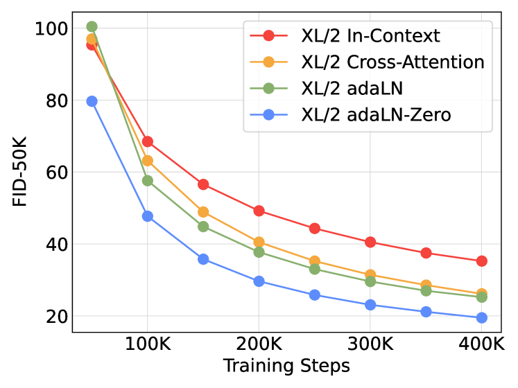
The headline empirical result (Figure 5): adaLN-Zero wins decisively on FID, despite being among the cheapest. Cross-attention costs 15% extra Gflops and is worse than adaLN-Zero. In-context conditioning is worst of all — at 400K iterations, in-context FID is roughly twice that of adaLN-Zero. So the DiT paper’s recommendation is unambiguous: pool the condition into a vector and drive adaLN-Zero with it. No cross-attention.

注入条件的四种 block 设计。 一旦图像变成 token 序列，问题就是怎么把噪声水平 \(t\) 和类别标签 \(c\) 喂给网络。DiT 论文显式考虑了四种变体——这正是 Figure 3 右半边那四个 panel：

1. In-context conditioning。 把 \(t\) 和 \(c\) 的嵌入作为两个额外 token 拼到输入序列上（类似 ViT 的 [CLS]）。让普通 self-attention 把它们和图像 token 一起混合；最后一个 block 之后再丢掉。Gflops 几乎为零。
2. Cross-attention block。 把 \(t\) 和 \(c\) 拼成长度为 2 的序列，与图像 token 序列保持分开。在每个 block 里 self-attention 之后插入一个 multi-head cross-attention 层，让图像 query 去 attend \((t, c)\) 的 key/value。开销大约比其他三种多 15% Gflops。
3. adaLN block。 把 block 里的 LayerNorm 全部换成自适应 LayerNorm：缩放 \(\gamma\) 和偏移 \(\beta\) 不再是固定参数，而是用一个小 MLP 从 \(t + c\) 的嵌入回归出来。同一对 \((\gamma, \beta)\) 广播到所有 token。四种里 Gflops 最低。
4. adaLN-Zero block。 与 adaLN 相同，但额外再回归一个维度级缩放 \(\alpha\)，作用于每条残差分支被加回主干之前。把 MLP 初始化为让 \(\alpha\) 起初为零——每个 block 在初始时是恒等映射，随训练逐步发挥作用，对应 ResNet / U-Net 训练里”零初始化残差”那类技巧。

主要实证结果（Figure 5）：adaLN-Zero 大幅胜出，尽管它是四种里最便宜的。Cross-attention 多花 15% Gflops，FID 却比 adaLN-Zero 差。In-context 最差——在 400K 迭代时，in-context 的 FID 大约是 adaLN-Zero 的两倍。所以 DiT 论文的建议毫不含糊：把条件池化成一个向量，用它驱动 adaLN-Zero。不用 cross-attention。

The figure below — Figure 3 of the paper, the most-cited DiT figure — puts the full pipeline (left) next to the four block variants (right) on one page.

下图——论文 Figure 3，DiT 最常被引用的那张图——把完整流水线（左）和四种 block 变体（右）画在一页上。

And the FID curves that decided it:

让 adaLN-Zero 胜出的 FID 曲线：

The full block, written out. With the choice settled, the canonical DiT block (used in every subsequent paper that says “DiT”) is:

where \((\gamma_1, \beta_1, \alpha_1, \gamma_2, \beta_2, \alpha_2) = \text{MLP}(t + c)\) and the MLP is zero-initialized so all \(\alpha\) start near zero. Note the structure: just Self-Attn → FFN, two LayerNorms replaced by adaLN, two residual scales — no cross-attention.

Scaling behavior. The paper sweeps four model configs × three patch sizes × FID at each checkpoint:

The headline scaling result: Gflops, not parameter count, predict FID. Halve the patch size and parameters barely change but Gflops 4× — and FID drops just as much as if you had grown the model. DiT-XL/2 reaches FID 2.27 on class-conditional ImageNet 256×256, beating all prior diffusion models at the time.

The legacy. The adaLN-Zero block became the universal backbone of modern image / video DiTs — Stable Diffusion 3, Sora, Wan, Cosmos-Predict2.5, and the 2B Cosmos-Predict2 model that Cosmos Policy fine-tunes are all built on it. But none of these systems is just DiT: every text-to-image / text-to-video model reintroduces cross-attention as a separate layer. The reason is a structural mismatch between class labels and text.

DiT’s \(c\) is a 1000-way one-hot — a categorical variable with no internal structure. The “embed it, feed adaLN” pipeline is lossless for that kind of conditioning: a single vector carries the entire label, and broadcasting one \((\gamma, \beta, \alpha)\) tuple to every image token is exactly the right behavior when the whole image is just “a golden retriever”. A natural-language prompt is the opposite kind of object. It has position (“a red cube on a blue cube”), dependencies (“the cat that the dog is chasing”), and count (“three apples”). All of these facts live in the relative arrangement of tokens. If you pool the T5 / CLIP token sequence into a single vector and only feed adaLN, those structural facts get smeared together and the model produces images with the right vibe but the wrong content — the classic “two cats on the left, one dog on the right” prompt that comes back with the wrong counts and positions.

Cross-attention restores the missing channel: image queries attend to the unpooled text token sequence and can route information to specific spatial positions. The compromise the field converged on is a block of the form Self-Attn → Cross-Attn(text) → FFN, with all three sub-layers wrapped in adaLN-Zero modulation driven by the timestep \(t\) together with a pooled text summary. So adaLN-Zero is not replaced — it absorbs the global signal (noise level, overall style) for free, while cross-attention handles the positional and compositional parts of the text that adaLN structurally cannot represent.

Some recent designs go a step further: SD3’s MMDiT and Flux merge the text token sequence directly into the same attention as the image tokens — one big joint self-attention rather than self + cross — while still keeping per-modality adaLN-Zero modulation. But the high-level division is the same in every variant: adaLN-Zero carries the conditioning that is uniform across all spatial positions, and attention to the unpooled text carries the conditioning that is position-specific. DiT settled the first half of the recipe; modern systems added the second.

完整的 block 写出来。 选定 adaLN-Zero 之后，标准 DiT block（之后所有自称”DiT”的论文用的那个）就是：

其中 \((\gamma_1, \beta_1, \alpha_1, \gamma_2, \beta_2, \alpha_2) = \text{MLP}(t + c)\)，MLP 零初始化使所有 \(\alpha\) 开始接近零。注意结构：就是 Self-Attn → FFN，两个 LayerNorm 换成 adaLN，加两个残差缩放——没有 cross-attention。

Scaling 行为。 论文扫了 4 种模型配置 × 3 种 patch size × 各个 checkpoint 的 FID：

主要 scaling 结论：预测 FID 的是 Gflops，不是参数量。把 patch size 减半，参数几乎不变，Gflops 翻 4 倍——FID 下降的幅度和直接放大模型差不多。DiT-XL/2 在 ImageNet 256×256 类别条件生成上达到 FID 2.27，当时压过所有先前扩散模型。

留下的范式。 adaLN-Zero block 成了现代图像 / 视频 DiT 的通用骨架——Stable Diffusion 3、Sora、Wan、Cosmos-Predict2.5、以及 Cosmos Policy 微调用的那个 2B Cosmos-Predict2 模型，全都建立在它之上。但它们没有一个只是 DiT：每个 text-to-image / text-to-video 模型都把 cross-attention 作为单独一层加了回来。原因是类别标签和文本之间的一个结构性错配。

DiT 里的 \(c\) 是一个 1000 类 one-hot——一个没有内部结构的类别变量。”先嵌入再喂 adaLN”这条流水线对它是无损的：一个向量就装得下整个标签；并且把同一组 \((\gamma, \beta, \alpha)\) 广播到每个图像 token，正好就是”整张图就是一只 golden retriever”这种条件下你想要的行为。但自然语言 prompt 是相反类型的对象：它有位置（”红色立方体在蓝色立方体上“）、依赖（”被狗追的那只猫“）、计数（”三个苹果”）。这些信息全都活在 token 之间的相对排列里。如果你把 T5 / CLIP 的 token 序列池化成一个向量再只喂给 adaLN，这些结构事实就会被抹平——模型生成的图像”氛围对了但内容错了”：”左边两只猫、右边一只狗”那种 prompt 出来的数目和位置就会乱。

Cross-attention 把缺失的通道补回来：图像 query 去 attend 未池化的文本 token 序列，从而把信息路由到特定的空间位置。整个领域收敛到的妥协方案是这样形式的 block：Self-Attn → Cross-Attn(text) → FFN，三个子层都被由噪声水平 \(t\) 加上一个池化后的文本摘要驱动的 adaLN-Zero 包裹。所以 adaLN-Zero 并没有被替换——它免费地吸收全局信号（噪声水平、整体风格），而 cross-attention 则负责文本里 adaLN 结构上没法表达的位置和组合部分。

最近的一些设计走得更远：SD3 的 MMDiT 和 Flux 直接把文本 token 序列并入图像 token 同一个 attention——一个大的联合 self-attention，而不是 self + cross 两层——同时仍然保留按模态分开的 adaLN-Zero 调制。但所有变体里高层划分都是一致的：adaLN-Zero 承载在所有空间位置都一致的那部分条件，而对未池化文本的 attention 承载与位置相关的那部分条件。DiT 解决了配方的前半，现代系统补上了后半。

The DiT discussion above keeps using self-attention and cross-attention as if they were obvious — worth a one-section reminder of how they actually differ, since the rest of this post (Cosmos’s text cross-attention, Fast-WAM’s MoT) leans on it. For the full ground-up walkthrough — single-layer attention, multi-head attention, and the encoder-decoder origin story — see the transformers post.

The mechanical difference is just where Q, K, V come from. A self-attention layer takes a single sequence \(X\) and projects it three ways: \(Q = X W^Q\), \(K = X W^K\), \(V = X W^V\). The output \(\text{softmax}(QK^\top / \sqrt{d}) V\) has the same shape as \(X\) — every token has been refined by reading every other token in the same sequence. A cross-attention layer takes two sequences: \(Q\) is projected from stream \(A\), but \(K\) and \(V\) are projected from stream \(B\). The math is identical (same softmax, same shape rule), but the output is A-shaped and is a weighted read of B. So self-attention is “tokens look at each other”; cross-attention is “stream A looks up stream B”.

Why ever use cross-attention instead of just concatenating and self-attending? Three practical reasons:

1. Asymmetric flow. Self-attention is symmetric: every token influences every other token. Cross-attention is one-way — stream A reads B, but B is unchanged. That asymmetry is what you want when one stream should condition on another: an image denoiser reading a frozen T5 encoder, where you don’t want image gradients flowing back into the language model.
2. Variable-length conditioning without paying \(O(N_A^2)\) on \(B\). If \(B\) is much shorter than \(A\) (a 77-token text prompt vs \(1{,}024\) image patches), full self-attention over the concatenation is \(O((N_A + N_B)^2)\), with most cells wasted on text-text or text-padding. Cross-attention is \(O(N_A \cdot N_B)\) — exactly the cells you need.
3. Modality boundaries. Cross-attention keeps the two streams structurally separate: their MLPs, LayerNorms, and positional encodings can differ. Forcing them into a single self-attention requires a shared embedding space, which is awkward when the two modalities live at very different scales.

Where this shows up in this post:

• Original Transformer (encoder-decoder). The canonical example: decoder tokens read encoder output via cross-attention. (deep-dive)
• DiT. Tested cross-attention as one of four conditioning variants — with \(c\) a one-hot, it lost to adaLN-Zero (see the DiT subsection above).
• Cosmos-Predict / Cosmos Policy. Image / video tokens read T5-XXL via cross-attention; this pathway is what carries the language instruction \(\ell\) at policy fine-tuning time.
• Fast-WAM. Its Mixture-of-Transformer is a generalized cross-attention: video DiT and action expert each keep their own MLPs and norms, but attention pools both modalities’ Q / K / V so each branch reads the other.

The point is that “use cross-attention” isn’t an architectural quirk — it’s the standard answer whenever two streams should talk without merging.

上面 DiT 那一节反复出现 self-attention 和 cross-attention 这两个词，像是不证自明的——值得用一节把它们到底有什么差别说清楚，因为本文后半（Cosmos 的文本 cross-attention、Fast-WAM 的 MoT）都建立在这个区分之上。如果想要单层、多头、以及它们在 encoder-decoder 里的起源那种从零开始的完整推导，可以看Transformer 那篇 blog。

机械层面的差别只在于 Q、K、V 来自哪里。 一个 self-attention 层接收一条序列 \(X\)，然后三路投影：\(Q = X W^Q\)、\(K = X W^K\)、\(V = X W^V\)。输出 \(\text{softmax}(QK^\top / \sqrt{d}) V\) 形状和 \(X\) 一样——每个 token 都通过读取同一条序列里的其他 token 得到精修。一个 cross-attention 层接收两条序列：\(Q\) 投影自流 \(A\)，但 \(K\) 和 \(V\) 投影自流 \(B\)。数学完全一样（同一个 softmax、同一套形状规则），但输出形状随 A，内容是对 B 的加权读取。所以 self-attention 是”token 之间彼此看”；cross-attention 是”流 A 去查流 B”。

为什么不直接拼起来做 self-attention？ 三个实际理由：

1. 非对称信息流。 Self-attention 是对称的：每个 token 都会影响每个 token。Cross-attention 是单向的——流 A 读 B，B 不变。当你希望一个流去条件化另一个流时（比如图像去噪器去读一个冻结的 T5 编码器，不希望图像梯度倒流回语言模型），这种不对称恰好是你想要的。
2. 变长条件，但不付 \(O(N_A^2)\) 在 \(B\) 上的代价。 如果 \(B\) 比 \(A\) 短得多（77 token 的文本 prompt vs \(1{,}024\) 个图像 patch），把它们拼起来跑完整 self-attention 是 \(O((N_A + N_B)^2)\)，大部分 cell 浪费在 text-text 或 text-padding 上。Cross-attention 只算 \(O(N_A \cdot N_B)\)——恰好是你需要的那些 cell。
3. 模态边界。 Cross-attention 把两条流在结构上保持分离：它们的 MLP、LayerNorm、位置编码都可以不一样。强行塞进一个 self-attention 则要求共享同一个嵌入空间，当两边量纲差异很大时这一点很别扭。

它在本文里出现在哪些地方：

• 原始 Transformer（encoder-decoder）。 经典例子：decoder 的 token 通过 cross-attention 去读 encoder 输出。（详细推导）
• DiT。 把 cross-attention 作为四种条件注入变体之一做了测试——但因为 \(c\) 是 one-hot，它输给了 adaLN-Zero（见上面的 DiT 小节）。
• Cosmos-Predict / Cosmos Policy。 图像 / 视频 token 通过 cross-attention 去读 T5-XXL；策略微调时承载语言指令 \(\ell\) 的就是这条通路。
• Fast-WAM。 它的 Mixture-of-Transformer 是 cross-attention 的广义形式：视频 DiT 和动作专家各自保留自己的 MLP 和 norm，但 attention 时把两边的 Q / K / V 汇总到一起，于是每一边都能读到对方。

要点是：”用 cross-attention” 并不是一个架构上的怪招——只要两条流需要互通而不合并，它就是标准答案。

Neither DDPM nor DiT natively processes text. Both are denoisers that map \((x_t, t, c)\) to a noise prediction; what \(c\) is depends on the system. The original DDPM was fully unconditional. The original DiT used ImageNet’s 1000 class labels — \(c\) was a 1000-way one-hot fed through the same MLP that emits the adaLN coefficients.

So where does language come in for modern image / video diffusion? The answer is: a separate, usually frozen, text encoder. Stable Diffusion 1.5 used CLIP; SDXL used CLIP+T5; Stable Diffusion 3, Sora, and Cosmos-Predict all use T5-XXL. The text encoder turns a prompt into an embedding sequence \(\ell\), and that sequence is injected into the denoiser through one (or both) of two routes:

1. adaLN / FiLM. Pool \(\ell\) to a single vector and feed it (alongside the noise level \(t\)) into the MLP that emits each block’s \((\gamma, \beta, \alpha)\). This is direct generalization of how class labels were handled in the original DiT.
2. Cross-attention. Keep \(\ell\) as a sequence, and let image patches attend to it via cross-attention layers inserted into each block. This is what SD 1.5 and Sora-class models do.

SD3’s MM-DiT goes further: text and image tokens share a joint attention pool, with separate MLPs but interleaved attention.

A subtle point worth making explicit: cross-attention is not part of the recommended DiT recipe. The DiT paper did consider it — it was one of the four conditioning variants — but the empirical comparison ranked it strictly worse than adaLN-Zero (worse FID, 15% extra Gflops). For class-conditional generation, where \(c\) is a one-hot vector, that ranking is decisive: pool, drive adaLN-Zero, done. Modern text-conditional DiTs put cross-attention back into the block, not because adaLN was wrong but because text is not a one-hot. The canonical text-to-video block — used in Sora, Cosmos-Predict, Wan, and what Cosmos Policy fine-tunes — is

with all three sub-layers wrapped by adaLN-Zero modulation driven by \(t\) (and optionally a pooled text embedding). adaLN-Zero is still the conditioning backbone; cross-attention is the additional mechanism for reading the text sequence — exactly the functionality the original DiT didn’t need because its conditioning had no sequential structure.

The conceptual point is that the denoising backbone is language-unaware. It just receives a vector of numbers. Prompt adherence improves by swapping in a smarter text encoder, not by training the diffusion model on more language. This is the structural opposite of autoregressive video models, where text and discrete video tokens live in the same vocabulary and a single decoder-only transformer attends over both jointly — no external text encoder needed. The price AR pays is sequential decoding and discrete-token quantization losses; the price diffusion pays is that “language understanding” is forever outsourced.

For Cosmos Policy, the implication is concrete: when the post-training loop reuses Cosmos-Predict2’s T5-XXL cross-attention pathway with the language instruction \(\ell\) (“pick up the red cup”), all the language understanding lives in T5-XXL — the DiT itself only sees the cross-attention output.

DDPM 和 DiT 本身都不处理文本。它们都只是去噪器：把 \((x_t, t, c)\) 映射到一个噪声预测；\(c\) 是什么取决于系统。DDPM 原始论文里完全无条件。DiT 原始论文用的是 ImageNet 的 1000 类标签——\(c\) 是一个 1000 维 one-hot，喂进与产出 adaLN 系数同一个 MLP。

那现代图像 / 视频扩散模型的语言能力从哪儿来？答案是：一个独立的、通常被冻结的 text encoder。SD 1.5 用 CLIP；SDXL 用 CLIP+T5；SD3、Sora、Cosmos-Predict 都用 T5-XXL。Text encoder 把 prompt 变成一条嵌入序列 \(\ell\)，然后通过下面两种途径之一（或两种）注入去噪器：

1. adaLN / FiLM：把 \(\ell\) 池化成一个向量，与噪声水平 \(t\) 一起喂进每个 block 中产出 \((\gamma, \beta, \alpha)\) 的 MLP。这是 DiT 原始论文处理类别标签的直接推广。
2. Cross-attention：保持 \(\ell\) 是一条序列，让 image patch 通过插入在每个 block 中的 cross-attention 层去读它。SD 1.5 和 Sora 一档模型走这条路。

SD3 的 MM-DiT 走得更远：text 和 image token 共享同一个 attention 池，MLP 各自独立、attention 交错。

一个值得明说的细节：cross-attention 并不在 DiT 推荐的方案里。DiT 论文确实考虑过它——是四种条件注入变体之一——但实证对比里 cross-attention 严格比 adaLN-Zero 差（FID 更高、且多花 15% Gflops）。对于类别条件生成、\(c\) 是 one-hot 的情况，结论是干脆的：池化、驱动 adaLN-Zero，到此为止。现代 text-conditional DiT 把 cross-attention 加回block，不是因为 adaLN-Zero 错了，而是因为文本不是 one-hot。Sora、Cosmos-Predict、Wan、以及 Cosmos Policy 微调的那条流水线，标准 block 长这样：

三个子层都被 \(t\)（可叠加一个池化文本向量）驱动的 adaLN-Zero 包裹。adaLN-Zero 仍然是条件注入的主干；cross-attention 是额外加的那一层，专门负责读文本序列——这个功能恰好是原始 DiT 不需要的，因为它的条件没有序列结构。

核心概念是：去噪 backbone 对语言一无所知。它只是收到一个数字向量。Prompt 跟随的好坏由换一个更聪明的 text encoder 来改善，而不是由让扩散模型多学语言来改善。这与自回归视频模型的结构是镜像对立的——AR 把文本和离散视频 token 放进同一个词表，一个 decoder-only transformer 就能联合处理两边，不需要外接 text encoder。AR 付出的代价是串行解码和离散 token 量化损失；扩散付出的代价是”语言理解”永远被外包。

对 Cosmos Policy 来说，这个区分很具体：当后训练复用 Cosmos-Predict2 的 T5-XXL cross-attention 通路接受语言指令 \(\ell\)（比如 “pick up the red cup”）时，所有的语言理解都活在 T5-XXL 里——DiT 自己只看到 cross-attention 的输出。

A video model parameterizes \(p(z_{1:T} \vert c)\) over a sequence of frame latents \(z_t\) given conditioning \(c\). There are two dominant ways to factorize this distribution.

Autoregressive video models factorize causally:

Each frame is generated conditioned on the previous frames. The frame latents are typically discrete tokens from a VQ-VAE. Representative works: VideoGPT (Yan et al. 2021), MAGVIT-v2 (Yu et al. 2023), VideoPoet (Kondratyuk et al. 2023). The training objective is the standard token cross-entropy. The architecture is a decoder-only transformer — the same one that backs LLMs.

Diffusion video models treat the entire clip as one tensor and denoise it jointly:

(where \(\tau\) indexes diffusion steps, distinct from frame index \(t\)). All frames are corrupted together with noise level \(\tau\), and a DiT denoises them in parallel. Representative works: Sora (OpenAI 2024), Stable Video Diffusion (Blattmann et al. 2023), the Cosmos World Foundation Model platform (NVIDIA 2025), and Cosmos-Predict2.5.

Trade-offs.

Where they meet. The line is blurring. Diffusion Forcing (Chen et al. 2024) trains a single transformer that denoises each frame at an independently sampled noise level — recovering AR generation as the limit where earlier frames have noise level 0 and later frames have noise level \(\tau\). Cosmos Policy’s “planning mode” is exactly this trick: clamp \((s, a)\) to clean and denoise \((s', V)\) — diffusion in the within-clip generative direction, autoregressive across decision steps. So in practice the modern frontier is block-autoregressive diffusion: diffuse within a chunk, autoregress between chunks.

视频模型参数化 \(p(z_{1:T} \vert c)\)，即在条件 \(c\) 下一段帧潜变量序列 \(z_t\) 的分布。这个分布有两种主流分解方式。

自回归视频模型做因果分解：

每一帧都基于前文条件生成。帧潜变量通常是 VQ-VAE 出来的离散 token。代表工作：VideoGPT (Yan et al. 2021)、MAGVIT-v2 (Yu et al. 2023)、VideoPoet (Kondratyuk et al. 2023)。训练目标是标准的 token 交叉熵。架构是 decoder-only Transformer——和 LLM 一样的那个。

扩散视频模型把整段视频当作一个张量联合去噪：

（这里 \(\tau\) 索引扩散步，与帧索引 \(t\) 区分）。所有帧以同一个噪声水平 \(\tau\) 一起被加噪，DiT 并行去噪。代表工作：Sora (OpenAI 2024)、Stable Video Diffusion (Blattmann et al. 2023)、Cosmos World Foundation Model 平台 (NVIDIA 2025)，以及 Cosmos-Predict2.5。

取舍。

它们在哪里汇合。 边界正在模糊。Diffusion Forcing (Chen et al. 2024) 训练一个单一 Transformer，对每一帧独立采样噪声水平进行去噪——当前面的帧噪声水平为 0、后面的帧为 \(\tau\) 时就退化为 AR 生成。Cosmos Policy 的”规划模式”正是这个套路：把 \((s, a)\) 固定为干净、对 \((s', V)\) 去噪——在 clip 内是扩散、跨决策步是自回归。所以现代前沿其实是块自回归扩散：chunk 内扩散，chunk 间自回归。

Side-by-side, the two pipelines look very different in motion. The figure below lets you step through generation in both: try advancing the step counter and watch how AR fills exactly one frame per pass (and stops only after \(T\) passes), while diffusion gradually denoises all frames at once over a fixed number of \(\tau\) steps. The attention masks above each panel are the structural reason: a triangular mask forces causality, full attention permits joint refinement.

两条流水线并排放在一起、跑起来看的时候差别很明显。下图让你逐步推进两侧的生成：拖动步数即可看到 AR 每个 pass 只填一帧（而且要 \(T\) 个 pass 才结束），而扩散在固定的 \(\tau\) 步内所有帧一起逐步去噪。每个 panel 上面的注意力掩码就是这种行为差异的结构原因：三角掩码强制因果，全注意力允许联合精修。

Flow Matching (Lipman et al. 2022) and the closely related Rectified Flow (Liu et al. 2022) take a different angle on continuous-time generative modeling. Instead of defining a stochastic forward process and learning the reverse score, flow matching defines a deterministic interpolation path from noise to data and learns its velocity.

The most common (rectified) flow path is the straight line:

Differentiate: \(\frac{d x_t}{d t} = x_1 - x_0\). So the ground-truth velocity along this path is \(x_1 - x_0\). The flow-matching loss simply regresses a velocity network onto this:

At sampling time, integrate the learned ODE \(\frac{dx}{dt} = v_\theta(x, t)\) from \(t=0\) (noise) to \(t=1\) (data), e.g. with Euler steps. Because the underlying paths are straight, you can integrate with very few steps — often \(5\)–\(10\) — vs hundreds for classical diffusion.

The objective looks almost identical to DDPM noise prediction, but it is actually predicting the velocity field of a probability flow, not noise. Cosmos-Predict2 and Fast-WAM both use this objective. For an extended discussion of flow matching as a generative-modeling framework — including its appearance as a policy class in deep RL — see the flow-matching-RL post.

Flow Matching (Lipman et al. 2022) 和与它紧密相关的 Rectified Flow (Liu et al. 2022) 给连续时间生成建模换了个角度。不再定义一个随机前向过程并学习反向分数，而是定义一条从噪声到数据的确定性插值路径，并学习这条路径的速度场。

最常用（rectified）的流路径就是一条直线：

求导：\(\frac{d x_t}{d t} = x_1 - x_0\)。所以这条路径上的真实速度就是 \(x_1 - x_0\)。流匹配损失就是把一个速度网络回归到它上面：

采样时，把学到的 ODE \(\frac{dx}{dt} = v_\theta(x, t)\) 从 \(t=0\)（噪声）积到 \(t=1\)（数据）即可，比如用 Euler 法。由于底层路径是直的，往往只要 \(5\)–\(10\) 步——而经典扩散需要数百步。

目标看起来和 DDPM 的噪声预测几乎一样，但它实际预测的是一条概率流的速度场，而不是噪声。Cosmos-Predict2 和 Fast-WAM 都用这个目标。关于 flow matching 作为生成建模框架的延伸讨论——包括它作为深度 RL 中策略类的用法——见flow-matching-RL 那篇 blog。

The two are not rival paradigms — they are different choices on the same continuous-time generative-modeling spectrum.

Both define a process linking a tractable prior \(p_0 = \mathcal{N}(0, I)\) to a data distribution \(p_1 = p_{\text{data}}\), parameterize a network on a noisy intermediate \(x_t\), and regress a target.

Where they differ:

The equivalence. Lipman et al. show that flow matching with a Gaussian probability path recovers score-based diffusion as a special case — DDPM’s \(x_t = \sqrt{\bar\alpha_t} x_0 + \sqrt{1-\bar\alpha_t}\, \epsilon\) is just a particular curved path between \(x_0\) and noise. Conversely, a flow-matching velocity field can be converted into a score, and vice versa, via the relationship \(\nabla \log p_t(x) = -\frac{1}{\sigma_t^2}(x - \sqrt{\bar\alpha_t}\, \mathbb{E}[x_0 \vert x_t])\).

Why flow matching is winning in practice. With straight paths, integrating the ODE for ~10 steps already reaches data quality; with diffusion’s curved paths, you typically need 50+ steps for the same fidelity. The training objective is also simpler: no \(\bar\alpha_t\) schedule, no signal-to-noise weighting tricks. Recent video models — Cosmos-Predict2, Wan2.1, and Fast-WAM — all use flow matching for these efficiency reasons. The whole “iterative video denoising” cost in imagine-then-execute WAMs is fundamentally a flow-matching ODE integration, and Fast-WAM’s central question — do we need to integrate this ODE at test time? — only makes sense once you see flow matching as the underlying machinery.

两者并非对立范式——它们是同一条连续时间生成建模光谱上的不同选择。

共同点： 二者都定义一个把可处理先验 \(p_0 = \mathcal{N}(0, I)\) 与数据分布 \(p_1 = p_{\text{data}}\) 连起来的过程，在带噪中间态 \(x_t\) 上参数化一个网络，并回归到某个目标。

不同点：

等价性。 Lipman 等人证明：当流匹配选择一条高斯概率路径时，会退化为基于分数的扩散——DDPM 的 \(x_t = \sqrt{\bar\alpha_t} x_0 + \sqrt{1-\bar\alpha_t}\, \epsilon\) 不过是 \(x_0\) 与噪声之间一条特定的弯曲路径。反过来，流匹配的速度场也能通过 \(\nabla \log p_t(x) = -\frac{1}{\sigma_t^2}(x - \sqrt{\bar\alpha_t}\, \mathbb{E}[x_0 \vert x_t])\) 这类关系转换成分数。

为什么流匹配在实践中胜出。 用直线路径时，积分 ODE 大约 10 步就能达到数据质量；用扩散的弯曲路径，往往需要 50+ 步才能达到同样保真度。训练目标也更简单：没有 \(\bar\alpha_t\) 调度，没有信噪比加权技巧。近期视频模型——Cosmos-Predict2、Wan2.1、Fast-WAM——都因为这些效率原因采用了流匹配。所谓 imagine-then-execute WAM 的”迭代视频去噪”开销，本质上就是流匹配 ODE 的积分；而 Fast-WAM 的核心问题——测试时还需要积这个 ODE 吗？——只有把流匹配看作底层机器之后才能问出来。

The geometric picture is the cleanest way to see the difference. Plot noise and data as two endpoints in some abstract space; each formulation traces a different trajectory between them, and that trajectory’s curvature is precisely what determines how many integration steps you need at sampling time. The figure below draws both paths in 2D and lets you slide \(t \in [0, 1]\) to watch the moving point and its velocity arrow on each.

要看清这个区别，几何视角是最干净的。把噪声和数据想象成某个抽象空间里的两个端点，每种方法都在它们之间画出一条不同的轨迹——而这条轨迹的弯曲程度，恰好决定了采样时需要多少积分步。下图把两条路径画在 2D 平面上，拖动 \(t \in [0, 1]\) 滑块即可看到每条路径上点的位置和它的速度向量。

A latent video diffusion model parameterizes \(p_\theta(z_{1:T} \vert o, l)\), where \(o\) is the conditioning observation, \(l\) is a language instruction, and \(z_{1:T}\) are latent frames produced by a spatiotemporal VAE. To turn this into a policy, we need to model

where \(a_{1:H}\) is an action chunk of horizon \(H\). There are essentially three design axes:

1. Where do actions live? Are they an extra “modality” inserted into the same diffusion sequence (Cosmos Policy), or do they live in a separate expert head that attends to the video stream (Fast-WAM)?
2. What does the joint loss factorize into? \(p(a, s' \vert s)\), \(p(s' \vert s, a)\), \(p(V(s') \vert s, a, s')\), etc. Different factorizations supply different gradients.
3. What runs at test time? Generate the future and read off actions (imagine-then-execute), or skip future generation entirely (action-only forward pass)?

The two papers below sit on different points of these axes.

潜空间视频扩散模型参数化 \(p_\theta(z_{1:T} \vert o, l)\)，其中 \(o\) 是条件观测，\(l\) 是语言指令，\(z_{1:T}\) 是由时空 VAE 产出的潜帧。要把它变成策略，我们需要建模

其中 \(a_{1:H}\) 是长度为 \(H\) 的动作块。本质上有三个设计维度：

1. 动作放在哪里？ 它是作为一个额外的”模态”插入到同一条扩散序列中（Cosmos Policy），还是放在一个独立的专家头里、通过注意力读取视频流（Fast-WAM）？
2. 联合损失如何分解？ \(p(a, s' \vert s)\)、\(p(s' \vert s, a)\)、\(p(V(s') \vert s, a, s')\) 等。不同分解提供不同的梯度。
3. 测试时跑什么？ 生成未来再读出动作（imagine-then-execute），还是完全跳过未来生成（仅动作前向传播）？

下面两篇工作处在这些维度的不同位置。

The framing. Cosmos brands itself as a World Foundation Model (WFM), not a World Action Model (WAM), and the choice is deliberate rather than cosmetic. A WFM is action-agnostic: it is pretrained purely on video — given some context (text, an image, a short clip), predict the future video. There is no action loss, no robot embodiment, no policy in the training objective. NVIDIA’s Cosmos paper (2025) positions the model as the video analog of an LLM foundation model: one large pretrained backbone over a massive video corpus, then a zoo of fine-tunes for specific downstream tasks.

WAM is downstream. A “World Action Model” is one of those downstream specializations: it predicts or generates actions, conditioned on observations, with an action loss in the training objective. Cosmos Policy is the WAM-shaped fine-tune of the Cosmos-Predict2 WFM — the backbone is reused, but the latent-slot layout is repurposed so that some slots carry actions and value, and the loss now includes action prediction. Fast-WAM is also a WAM by this definition: its “video” branch is a co-training auxiliary, but the main inference output is actions. The clean two-part test for “is this a WAM?” is (a) does the inference graph emit actions, and (b) is the action loss in the training objective?

Why the distinction matters. A WFM is what you scale — it gets the foundation-model treatment of “more data, more compute, more parameters”. A WAM is what runs on a robot — its capability ceiling is set by its WFM backbone, but the deployment characteristics (latency, accuracy, sample efficiency) are determined by the WAM-side design choices: latent layout, masking pattern, whether actions live in the main sequence (Cosmos Policy) or in a separate expert (Fast-WAM), and what runs at test time. Cosmos Policy and Fast-WAM are two points in WAM design space; in principle either could sit on top of any sufficiently capable WFM. Calling Cosmos itself a “WFM” rather than a “WAM” reserves the WFM label for the generic video pretraining and lets each downstream task — policy, simulator, evaluator, planner — claim its own model name.

这是一个刻意的框架选择。 Cosmos 把自己叫 World Foundation Model（WFM）而不是 World Action Model（WAM），是一个有意的命名选择，不是市场修辞。WFM 是与动作无关的：它纯粹在视频上预训练——给定某种上下文（文本、单帧图像、短片段），预测未来视频。训练目标里没有动作损失、没有机器人本体、没有策略。NVIDIA 的 Cosmos 论文（2025）把这个模型定位为视频版的 LLM foundation model：一个在海量视频语料上预训练的大主干，配上一组针对各类下游任务的微调。

WAM 是下游。 “World Action Model” 就是这些下游专门化里的一种：它预测或生成动作，以观测为条件，训练目标里有动作损失。Cosmos Policy 就是 Cosmos-Predict2 这个 WFM 的 WAM 形态微调——主干被复用，但潜槽布局被改造，让一些槽位承载动作和价值，loss 里加上了动作预测。按这个定义，Fast-WAM 同样是 WAM：它的”视频”分支是联合训练的辅助任务，但推理时的主输出是动作。判断一个模型是不是 WAM 最干净的两条标准是：(a) 推理图是否输出动作？(b) 训练目标里是否包含动作损失？

这个区分为什么重要。 WFM 是用来做 scale 的——它享受 foundation-model 那一套”更多数据、更多算力、更多参数”的待遇。WAM 是真正跑在机器人上的——它的能力上限由其 WFM 主干决定，但部署特性（延迟、准确率、样本效率）由 WAM 端的设计选择决定：潜空间布局、掩码模式、动作是放在主序列里（Cosmos Policy）还是放在独立的 expert 里（Fast-WAM）、以及测试时跑什么。Cosmos Policy 和 Fast-WAM 是 WAM 设计空间里的两个不同点；理论上两者都可以建立在任何足够强的 WFM 主干之上。把 Cosmos 本身叫 “WFM” 而不是 “WAM”，正是为了把 WFM 这个标签留给通用的视频预训练，让每个下游任务（策略、模拟器、评估器、规划器）都能各自命名为自己的那种模型。

Cosmos Policy’s distinguishing choice is one backbone, many slots. It takes a pretrained 2B Cosmos-Predict2 video DiT, leaves the architecture untouched, and post-trains it by repurposing some of the latent slots to carry actions, proprioception, and value instead of pure video. The same DiT then handles policy, world model, and value prediction by switching which slots are masked clean vs noised. The next three subsections walk through the latent layout, the joint loss, and what the inference graph looks like in the two deployment modes.

Cosmos Policy 的核心选择是一条主干、多种槽位。它拿一个预训练好的 2B Cosmos-Predict2 视频 DiT，架构原封不动，通过后训练把其中一些潜槽改作他用——承载动作、本体感觉和价值，而不是纯视频。同一个 DiT 通过切换”哪些槽干净、哪些槽加噪”，就能扮演策略、世界模型、价值模型三种角色。下面三小节依次讲潜空间布局、联合 loss、以及两种部署模式下的推理图。

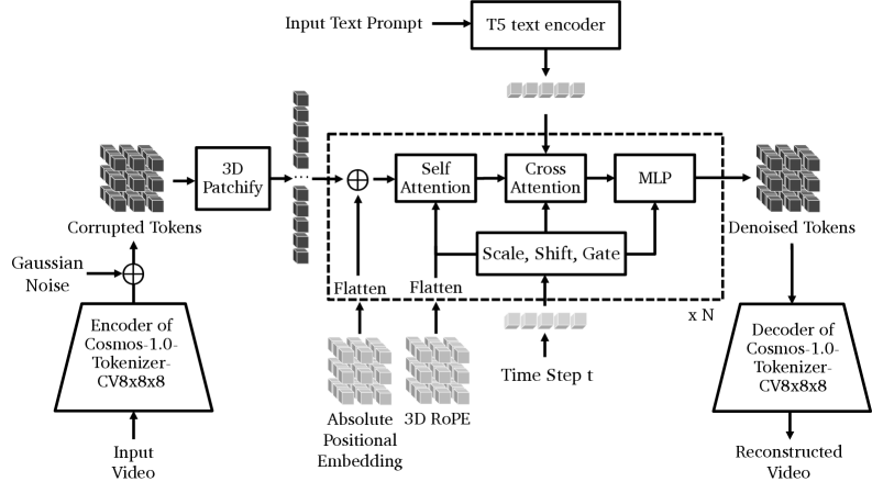
Before walking through what Cosmos Policy adds, it helps to anchor on what the base Cosmos-Predict architecture looks like. The figure below — reproduced from the Cosmos World Foundation Model paper (NVIDIA 2025) — shows the standard text-to-video DiT pipeline that Cosmos Policy fine-tunes: a Cosmos-Tokenize1 spatiotemporal VAE encodes the input video into latent tokens, Gaussian noise is added, and the tokens flow through 3D patchify and a stack of (N) DiT blocks. Each block follows the adaLN-Zero recipe — Self-Attention → Cross-Attention → MLP, with Scale/Shift/Gate driven by the time step (t) — plus T5-XXL text cross-attention. The denoised tokens are decoded back to pixels by the same VAE.

在讲 Cosmos Policy 加了什么之前，先把 Cosmos-Predict 基础架构看清楚是有帮助的。下图——出自 Cosmos World Foundation Model 论文 (NVIDIA 2025)——展示的是 Cosmos Policy 微调时复用的那条标准 text-to-video DiT 流水线：Cosmos-Tokenize1 时空 VAE 把输入视频编码成潜 token，加上高斯噪声后，token 经过 3D patchify 进入由 (N) 个 DiT block 组成的堆栈。每个 block 都是 adaLN-Zero 套路——Self-Attention → Cross-Attention → MLP，Scale/Shift/Gate 由时间步 (t) 驱动——再加上 T5-XXL 文本 cross-attention。去噪后的 token 通过同一个 VAE 解码回像素。

The base model is Cosmos-Predict2-2B, a flow-based latent video diffusion transformer using the Wan2.1 spatiotemporal VAE and an EDM denoising objective. Cosmos Policy’s design choice is deliberately conservative: no new architectural components. Instead, every additional modality is encoded as a latent frame and inserted into the diffusion sequence.

For a multi-camera robot, the sequence carries 11 latent frames:

Everything — proprioception, wrist and third-person camera frames, the action chunk, the predicted future state, and a learned value head — is denoised under the same diffusion transformer. The action chunk gets its own latent slot but is structurally indistinguishable from a video frame; the model’s attention machinery, positional encodings, and noise schedule are reused as-is.

This is a strong stance on representation: actions, observations, and values are all “frames” in the same latent video, and any factorization is induced by which frames are clean vs. noisy at inference.

基础模型是 Cosmos-Predict2-2B，一个基于 flow 的潜空间视频扩散 transformer，使用 Wan2.1 时空 VAE 和 EDM 去噪目标。Cosmos Policy 的设计选择刻意保守：不加任何新的架构组件。取而代之，每一个额外模态都被编码为一个潜帧并插入扩散序列。

对于多相机机器人，整条序列包含 11 个潜帧：

一切——本体感觉、腕部和第三人称相机帧、动作块、预测的未来状态、学到的价值头——都在同一个扩散 transformer 下被去噪。动作块占据自己的潜槽，但在结构上与一个视频帧无异；模型的注意力机制、位置编码、噪声调度全部原样复用。

这是一个强表示立场：动作、观测、价值在同一段潜空间视频中都是”帧”，任何分解只取决于推理时哪些帧是干净的、哪些是带噪的。

The first thing to nail down is how a robot’s heterogeneous inputs — RGB cameras, joint angles, action vectors, scalar values — all end up looking like the same kind of object inside the model. The figure below traces each modality’s pathway: RGB goes through the pretrained Wan2.1 VAE, while every scalar stream just gets normalized and tile-broadcast into a \(H' \times W' \times 16\) volume. The point is the convergence at the right column — every input lands at the identical shape.

首先要搞清楚的是：机器人的异构输入——RGB 相机、关节角度、动作向量、标量价值——在模型内部是怎么变成同一种东西的。下图把每种模态的路径都画了出来：RGB 走预训练的 Wan2.1 VAE，所有标量流则只是归一化加 tile 广播成一个 \(H' \times W' \times 16\) 的体积。关键在于右侧那一列的汇聚——每种输入最终都落到完全相同的形状。

Once every modality is the same shape, “what task am I doing” reduces to “which slots are clean vs noised.” The figure below makes this concrete: the 11-slot layout stays fixed, and three different masking patterns turn the same backbone into a policy, a world model, or a value head. Click any of the training-mode buttons to see the corresponding mask, and watch which gradient term in the update equation lights up.

一旦所有模态形状一致，”我在做哪个任务”就退化为”哪些槽位是干净的、哪些是带噪的”。下图把这一点画清楚：11 个槽位的布局始终不变，三种不同的掩码模式让同一个主干变成策略、世界模型或价值头。点击任意训练模式按钮即可看到对应的掩码，并观察更新公式中哪个梯度项被高亮。

A single batch is split across three conditional factorizations. With \(s\) the current state, \(a\) the action chunk, and \(s'\) the resulting state:

• 50% — policy: \(p_\theta(a, s', V(s') \vert s)\), trained on demonstrations.
• 25% — world model: \(p_\theta(s', V(s') \vert s, a)\), trained on rollouts.
• 25% — value model: \(p_\theta(V(s') \vert s, a, s')\), trained on rollouts.

Each factorization is implemented by clamping the corresponding latent frames to clean (zero noise) and noising the rest. Because the network is the same diffusion transformer, the three losses share gradients — the policy benefits from gradients computed on rollout-only world-model and value-model objectives.

Two practical knobs matter:

1. The default Cosmos noise distribution (log-normal) is replaced with a 70/30 hybrid log-normal–uniform split, biasing samples toward higher noise levels — the regime where the model has to actually predict, not just denoise a near-clean image.
2. Inference noise lower bound is raised from \(\sigma_{\min}=0.002\) to \(\sigma_{\min}=4\), terminating denoising early. Combined with parallel decoding of all latent slots, this lets the policy run in 5 denoising steps on LIBERO/RoboCasa.

单个 batch 被切分到三种条件分解上。记 \(s\) 为当前状态、\(a\) 为动作块、\(s'\) 为下一状态：

• 50% — 策略：\(p_\theta(a, s', V(s') \vert s)\)，在示范上训练。
• 25% — 世界模型：\(p_\theta(s', V(s') \vert s, a)\)，在 rollout 上训练。
• 25% — 价值模型：\(p_\theta(V(s') \vert s, a, s')\)，在 rollout 上训练。

每种分解都通过把对应潜帧固定为干净（零噪声）、其余加噪来实现。由于使用的是同一个扩散 transformer，三种损失共享梯度——策略从仅在 rollout 上计算的世界模型和价值模型目标的梯度中受益。

两个工程旋钮值得注意：

1. 默认 Cosmos 噪声分布（log-normal）被替换为 70/30 的 log-normal–均匀混合分布，把样本偏向更高噪声水平——这才是模型必须真正预测、而不是只去噪一张近乎干净的图像的区间。
2. 推理时噪声下界从 \(\sigma_{\min}=0.002\) 提到 \(\sigma_{\min}=4\)，提前终止去噪。结合所有潜槽的并行解码，这让策略在 LIBERO/RoboCasa 上只需 5 步去噪。

“Shared gradients” is shorthand for parameter sharing. The three losses are not literally the same gradient vector — they compute different things on different batch subsets. What is shared is the set of parameters \(\theta\) that all three gradients update:

Why it matters: if the three objectives ran on three separate networks, rollout-only gradients (\(\mathcal{L}_{\text{wm}}, \mathcal{L}_{\text{val}}\)) would only improve their own networks and give the policy nothing. Because Cosmos Policy stuffs all three factorizations into a single diffusion transformer — switched only by which latent frames are clamped clean vs. noised — the visual and dynamics features learned on rollout data flow directly into the policy backbone. The policy ends up training on 100% of the data: 50% demonstrations directly, 50% rollouts indirectly through shared representations.

This is standard multi-task learning, but Cosmos Policy takes it to an extreme: even “which task am I doing” is encoded purely in the noise pattern over latent slots; the network itself is task-agnostic.

“共享梯度”是参数共享的一种简称。三个损失在文字上不是同一个梯度向量——它们在不同 batch 子集上计算不同的目标。真正被共享的，是三个梯度都去更新的同一组参数 \(\theta\)：

为什么这么做有意义：如果三个目标分别有各自的网络，那么仅在 rollout 数据上计算出来的 \(\mathcal{L}_{\text{wm}}, \mathcal{L}_{\text{val}}\) 梯度只能改进它们自己的网络，对策略毫无帮助。而 Cosmos Policy 把三种分解全部塞进同一个扩散 transformer——区分它们的只是”哪些潜帧固定为干净、哪些被加噪“——于是在 rollout 数据上学到的视觉与动力学特征直接流入策略的主干。最终的策略实际上在 100% 的数据上训练：50% 示范直接、50% rollout 通过共享表示间接。

这就是标准的多任务学习，只是 Cosmos Policy 把它推到了极端：连”我在做哪个任务”都只通过潜槽上的噪声模式编码；网络本身对此一无所知。

Cosmos Policy runs in two modes:

• Direct mode — clamp the current state \(s\) to clean, parallel-denoise the action, future state, and value slots. No VAE decoding — the future state is consumed in latent space only. ~5 denoising steps; real-time on a single GPU.
• Planning mode — sample \(N\) action proposals; for each, autoregressively predict \(s'\) and \(V(s')\); pick the proposal with the highest predicted value. This is best-of-\(N\) planning inside a single foundation model. With 3 future-state predictions × 5 value predictions per proposal, end-to-end latency is ~5 s per chunk.

Empirically, planning mode buys +12.5 points on the harder ALOHA tasks but is overkill on LIBERO/RoboCasa, where direct mode already saturates. Headline numbers:

Ablations: removing auxiliary losses costs 1.5%; training from scratch (no Cosmos-Predict2 init) costs 3.9% on LIBERO — so most of the lift is post-training, not pretraining, but pretraining is not free either.

Cosmos Policy 有两种推理模式：

• 直接模式——把当前状态 \(s\) 固定为干净，对动作、未来状态、价值槽并行去噪。不做 VAE 解码——未来状态只在潜空间被消费。约 5 步去噪；单卡实时。
• 规划模式——采样 \(N\) 个动作候选；对每个候选自回归地预测 \(s'\) 和 \(V(s')\)；选预测价值最高者。这是在单个基础模型内部做 best-of-\(N\) 规划。每个候选 3 次未来状态预测 × 5 次价值预测，端到端约 5 秒一个 chunk。

经验上，规划模式在更难的 ALOHA 任务上带来 +12.5 分，但在 LIBERO/RoboCasa 上是过度——直接模式已经饱和。主要数字：

消融：去掉辅助损失掉 1.5%；不从 Cosmos-Predict2 初始化（从头训练）在 LIBERO 上掉 3.9%——所以主要提升来自后训练而非预训练，但预训练也并非可有可无。

Fast-WAM takes a different stance. Instead of one DiT handling everything, it splits video and action into two experts coupled by a single shared attention layer, and asks whether the video branch needs to actually run iterative denoising at test time at all. The answer is: train it as a co-training auxiliary, then drop the future-video denoising loop at inference. The five subsections below cover the motivating question, the Mixture-of-Transformer architecture, the inside of “shared attention”, the single-pass inference graph, and the ablation that decides between the three WAM paradigms.

Fast-WAM 走的是另一条路线。它不让一个 DiT 包揽一切，而是把视频和动作拆成两个专家，靠一层共享 attention 耦合，并且追问：测试时视频分支到底需不需要真的做迭代去噪？回答是：训练时把视频损失当 co-training 辅助任务保留，推理时整段去噪循环跳过。下面五小节依次讲：动机问题、Mixture-of-Transformer 架构、共享 attention 内部、单次前向的推理图、以及在三种 WAM 范式中作出裁决的关键消融。

Most prior WAMs (UniVLA, WorldVLA, and Cosmos Policy in its planning mode) follow an imagine-then-execute pipeline: at every action step, run iterative video denoising to hallucinate future frames, then read off (or condition on) actions. The runtime cost of denoising a future video is the dominant inference bottleneck — typically several hundred milliseconds to seconds per chunk.

Fast-WAM’s central question is uncomfortably basic: do we actually need the imagined video at test time, or is it only useful during training as a representation-learning auxiliary?

此前大多数 WAM（UniVLA、WorldVLA，以及 Cosmos Policy 的规划模式）都遵循 imagine-then-execute 流程：每个动作步上，跑迭代式视频去噪幻想未来帧，再据此读出（或条件化）动作。去噪未来视频的运行时开销是推理的主要瓶颈——通常一个 chunk 要几百毫秒到数秒。

Fast-WAM 的核心问题朴素得令人不适：测试时我们到底需不需要被想象出的视频？还是说它只在训练时作为一个表示学习辅助任务有用？

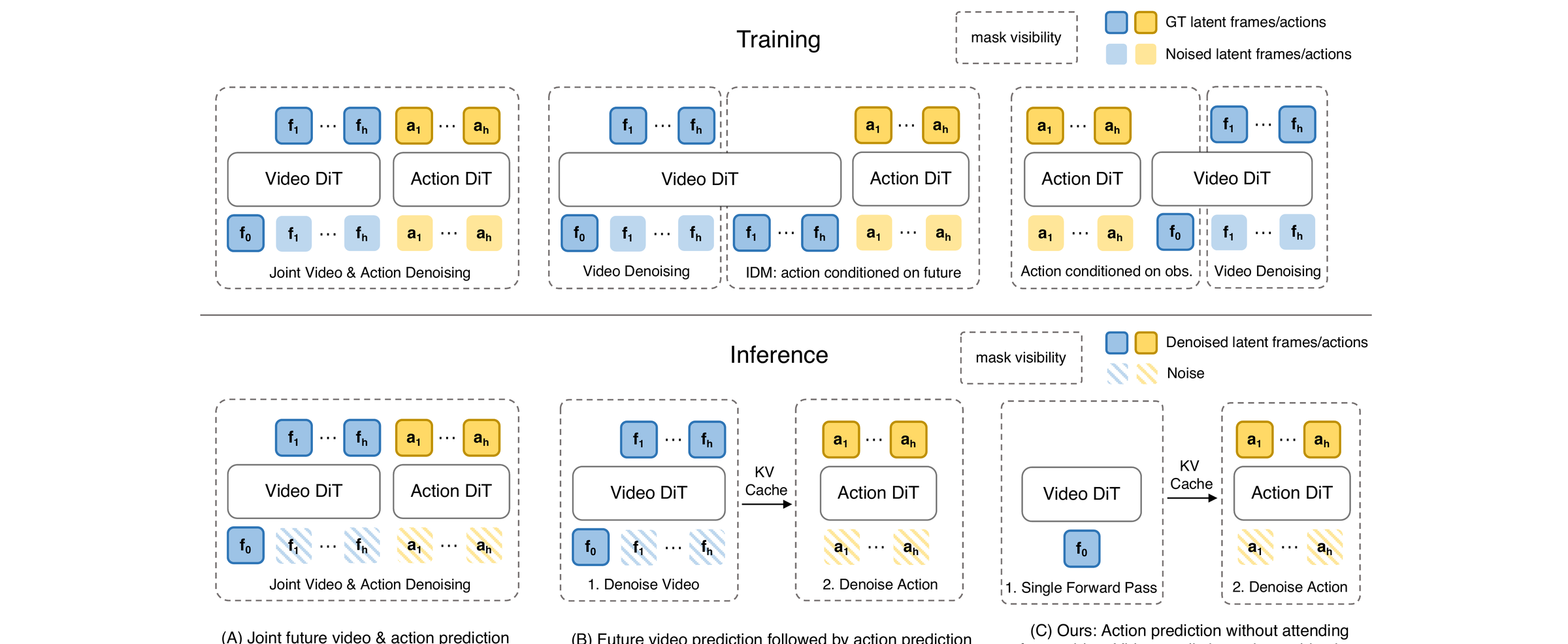
The paper draws a clean taxonomy of WAM paradigms before introducing its own. The figure below — Figure 1 of the Fast-WAM paper — contrasts the three: (A) joint-modeling WAMs that denoise video and action tokens together, (B) causal WAMs that first generate future observations and then condition action prediction on them, and (C) Fast-WAM, which keeps video co-training during training but skips the future-generation step at inference.

论文先把 WAM 的几种范式分得很清楚，再把自己的方案放进来。下图——Fast-WAM 论文的 Figure 1——对比了三种范式：(A) 联合建模 WAM，把视频与动作 token 一起去噪；(B) 因果 WAM，先生成未来观测、再让动作预测条件化在它上面；(C) Fast-WAM，训练时保留视频联合训练，但推理时跳过未来生成那一步。

The three columns are worth walking through, because the rest of the section is structured as Fast-WAM’s argument against (A) and (B).

(A) Joint-modeling WAMs. Video and action are both denoising targets in a single diffusion process. One backbone denoises the concatenated \((z_{1:T},\, a_{1:H})\) sequence — at every denoising step \(\tau\), both the future-video latents and the action chunk are partially denoised, and they evolve together along one trajectory. Action tokens attend to (still-noisy) video tokens through joint attention, so the model refines actions based on a partially-imagined future. Symmetric coupling: action also influences video. Cost at inference: every action prediction needs a full multi-step denoise over both modalities — typically \(10\)–\(50\) steps, each step touching all video + action tokens. For a 9-frame future at 8×8 latent resolution this is by far the dominant compute. Cosmos Policy’s joint training is the closest representative of this stance (it uses three masking patterns over a single backbone rather than literal concatenation, but the spirit — one DiT, both modalities denoised together — is the same).

(B) Causal WAMs. Inference is split into two stages with a clean causal direction: stage 1 is a video diffusion model that denoises \(z_{1:T}\) from noise into clean future frames conditioned on the current observation \(o\) and language \(l\); stage 2 is a (typically much smaller) action policy that takes the generated future frames as extra context and produces \(a_{1:H}\), usually in a single pass or a small handful of steps. The “execute” stage is cheap; the “imagine” stage is not. Information flow is one-way: video → action, never action → video. Cost at inference: dominated by stage 1’s full video denoise; stage 2 adds only a small fixed overhead. Representatives: UniVLA, WorldVLA — and Cosmos Policy’s planning mode is also a Causal WAM (it imagines future frames in a first denoising pass and then reads off actions).

Why does the IDM training cell look different from its inference cell in the figure? Because training has a luxury inference does not: the real future frames sit in the dataset. So at training time the action head is conditioned on clean ground-truth future frames — a supervised inverse-dynamics task (“given \(o\), \(o'\), what action \(a\) produced this transition?”) — while the video DiT is separately trained to denoise future frames from noise. At inference the GT future is gone (the agent has to act to produce that future), so stage 1 has to hallucinate the future by iterative denoising, and only then can the action head read off frames. Training conditions on real futures; inference conditions on generated ones. This asymmetry is the structural weakness of IDM-style WAMs: the action head only ever saw clean GT futures during training, but at deployment it sees diffusion-generated futures that may be subtly off. It is also why inference is unavoidably expensive — you cannot shortcut the future-generation step, because the action head was never trained to be robust to a bad future.

(C) Fast-WAM. Training looks like (A): both the action flow-matching loss and the video flow-matching loss are active, and the shared attention carries gradient between branches. But at inference the video pathway runs once on the clean first observation only, and the future-video denoising loop is skipped entirely. The 1B action expert is the only thing that iterates (10 steps, CFG = 1.0). Information flow at deployment is asymmetric: the video branch is a fixed key/value bank, the action expert queries it. Cost at inference: one cheap clean pass through the 5B video DiT plus 10 cheap action denoising steps — the paper reports 190 ms total, ~4× faster than (A)- or (B)-style baselines. The bet: whatever the world model has learned has already left its imprint on the shared attention parameters by the time training ends; re-rolling out video at test time is paying twice for the same insight.

A note on layout: in (C), Action DiT is on the left at training but on the right at inference — left/right means different things in each row. Training is parallel (both branches run together, sharing attention), so left-right is just “which loss owns which branch”. Inference is serial (video DiT runs once → K/V cache → action DiT iterates), so left-to-right is execution order. And the actual difference between (A) and (C) is that (A) joint-trains the two as one denoising system over \((z, a)\), while (C) does not — in (C) action is the primary task and video is a parallel co-training auxiliary, not a joint diffusion target.

So the figure is really one axis — where in the lifecycle does video denoising happen? In (A) and (B) it happens at every test-time action step; in (C) only at training. The whole empirical contribution of the paper is the head-to-head comparison against (A)- and (B)-style ablations, holding the data and backbone fixed (see the decisive ablation below).

图里这三列值得一列一列走一遍，因为本节后半部分基本是 Fast-WAM 对 (A)、(B) 的论证。

(A) 联合建模 WAM。 视频和动作都是同一个扩散过程里的去噪目标。一个主干对拼接好的 \((z_{1:T},\, a_{1:H})\) 序列做去噪——每一步 \(\tau\)，未来视频潜变量与动作 chunk 都被部分去噪，沿同一条轨迹一起演化。动作 token 通过联合注意力读到（仍带噪的）视频 token，于是模型可以基于部分想象的未来来精修动作。耦合是对称的：动作也会反过来影响视频。推理代价：每次动作预测都要在两个模态上做一次完整多步去噪——通常 \(10\)–\(50\) 步，每步都要处理全部视频 + 动作 token。9 帧未来 × 8×8 潜分辨率，光这部分就吃掉绝大部分算力。Cosmos Policy 的联合训练最接近这种立场（它用单主干上的三种掩码模式，而不是字面意义上的拼接，但精神——一个 DiT 把两种模态一起去噪——是一样的）。

(B) 因果 WAM。 推理分两段，方向是干净因果的：第 1 段是视频扩散模型，把 \(z_{1:T}\) 从噪声去噪到干净未来帧，条件是当前观测 \(o\) 和语言 \(l\)；第 2 段是一个（通常小得多的）动作策略，把生成出来的未来帧作为额外上下文，输出 \(a_{1:H}\)，通常一遍前向就好或者少量几步。”execute” 这一段便宜，”imagine” 那一段不便宜。信息流是单向的：视频 → 动作，没有动作 → 视频。推理代价：主导项是第 1 段的完整视频去噪；第 2 段只是固定的小开销。代表：UniVLA、WorldVLA——以及 Cosmos Policy 的规划模式同样是因果 WAM（先在第一遍去噪里想象未来帧，然后读出动作）。

为什么图里 IDM 的训练格子和推理格子不一样？ 因为训练阶段有一个推理时不存在的奢侈品：真实的未来帧就摆在数据集里。所以训练时动作头的条件是干净的 ground-truth 未来帧——这是一个有监督的逆动力学任务（”给定 \(o\)、\(o'\)，是什么动作 \(a\) 产生了这个转移？”）——而视频 DiT 是单独学怎么把未来帧从噪声里去噪。推理时 GT 未来没有了（agent 必须通过行动来产生那个未来），所以第 1 段必须幻想出未来（迭代去噪），动作头才有未来帧可读。训练时的条件是真的，推理时的条件是生成的。这种不对称恰恰是 IDM 风格 WAM 的核心结构性弱点：动作头在训练时只见过干净 GT 未来，部署时却只看到扩散生成、可能略有偏差的未来。这也解释了为什么推理代价绕不开——没法跳过”生成未来”那一步，因为动作头从来没被训练成对差未来鲁棒。

(C) Fast-WAM。 训练看起来像 (A)：动作 flow-matching 损失与视频 flow-matching 损失都激活，共享 attention 把梯度在两个分支间传递。但推理时视频通路只在干净的首帧观测上跑一次，未来视频的去噪循环完全跳过。迭代去噪的只有 1B 的动作专家（10 步，CFG = 1.0）。部署时的信息流是不对称的：视频分支是一个固定的 key/value 仓库，动作专家来查询它。推理代价：5B 视频 DiT 跑一次干净前向，加 10 步便宜的动作去噪——论文报告总共 190 ms，比 (A)- / (B)- 风格的基线快约 4×。赌注：世界模型学到的一切，在训练结束时其实已经印在共享 attention 参数里了；测试时再 roll out 一遍视频，是在为同一个洞察付两次钱。

关于布局：(C) 里 Action DiT 训练行在左、推理行在右——两行的左右含义不一样。 训练是并行的（两分支同时跑、共享 attention），左右只是在交代”哪个 loss 管哪个分支”；推理是串行的（视频 DiT 先跑一次 → K/V cache → 动作 DiT 迭代），左到右就是执行顺序。而 (A) 和 (C) 的真正区别是：(A) 把两者当成一个 \((z, a)\) 上的联合去噪系统一起训；(C) 不是——(C) 里动作是主任务，视频是并行的 co-training 辅助，不是联合扩散目标。

所以这张图其实只有一个轴——视频去噪发生在生命周期的哪一段？在 (A) 和 (B) 里它发生在每一个测试时动作步上；在 (C) 里只发生在训练阶段。论文全部的实证贡献就是在数据和主干完全相同的前提下，把 Fast-WAM 与 (A)、(B) 风格的消融做正面对比（见下面的决定性消融）。

Fast-WAM uses a Mixture-of-Transformer (MoT): a 5B-parameter video DiT and a 1B-parameter action expert DiT, coupled by shared attention — the two experts run their own MLPs and norms but attend to a common token sequence. Inputs are partitioned by modality:

• Video tokens flow through the video DiT.
• Action tokens flow through the action expert.
• Both attend to each other through shared attention.

The training objective is a joint flow-matching loss

with \(\mathcal{L}_{\text{act}} = \mathcal{L}_{\text{FM}}(a_{1:H})\) on action chunks (horizon \(H = 32\)) and \(\mathcal{L}_{\text{vid}} = \mathcal{L}_{\text{FM}}(z_{1:T})\) on future video latents (9 frames after 4× temporal downsampling).

Fast-WAM 使用 Mixture-of-Transformer (MoT)：一个 5B 参数视频 DiT 加一个 1B 参数动作专家 DiT，二者通过共享注意力耦合——两个专家各自跑自己的 MLP 和 norm，但对一条共同的 token 序列做注意力。输入按模态划分：

• 视频 token 流经视频 DiT。
• 动作 token 流经动作专家。
• 二者通过共享注意力互相读到对方。

训练目标是联合 flow-matching 损失

其中 \(\mathcal{L}_{\text{act}} = \mathcal{L}_{\text{FM}}(a_{1:H})\) 作用于动作块（horizon \(H = 32\)），\(\mathcal{L}_{\text{vid}} = \mathcal{L}_{\text{FM}}(z_{1:T})\) 作用于未来视频潜（4× 时间下采样后 9 帧）。

The phrase “shared attention” is doing a lot of work in the architecture description above. The mechanic, concretely, is attention is shared but everything else is per-modality. Each MoT block does this:

1. Per-modality input projections. Video tokens \(x^v\) and action tokens \(x^a\) each go through their own QKV projection matrices: \(Q^v = x^v W_Q^v\), \(K^v = x^v W_K^v\), \(V^v = x^v W_V^v\), and similarly \((Q^a, K^a, V^a)\) from \(x^a\) via \(W_{Q,K,V}^a\). Each modality first lands in its own subspace.

2. Concatenate, then attend jointly. The Q, K, V tensors are concatenated along the sequence dimension into one combined Q, K, V, and standard self-attention runs on the combined sequence:

A video token’s query attends to both video and action keys/values; an action token’s query attends to both as well. This is the only operation that mixes modalities.

1. Split back, apply per-modality output side. The attention output is split back along the sequence dimension into video-shaped and action-shaped outputs, each of which goes through its own output projection \(W_O^v\) or \(W_O^a\), residual connection, LayerNorm, and MLP. Block ends.

So “shared” = a single attention computation pools both modalities’ Q/K/V; “not shared” = everything outside the attention math (input projections, output projection, LayerNorm, MLP) is duplicated per modality.

The figure below draws one MoT block end-to-end with the per-modality (pink) and shared (blue) parts labeled separately. Read it bottom-to-top: video and action tokens enter, each goes through its own QKV projection, the resulting Q / K / V tensors are concatenated, one shared softmax computes attention over the joint sequence, the output is split back per modality, and each side runs through its own output projection / FFN / LayerNorm before exiting. The MoT paper (Liang et al. 2024) calls this design modality-aware sparsity; the actual “shared” piece is just the scaled-dot-product softmax in the middle.

“共享 attention” 这个词在上面的架构描述里干了不少活。具体的机制就一句话：attention 共享，attention 之外的东西每个模态都是自己一套。每个 MoT block 内部是这样的：

1. 按模态分开的输入投影。 视频 token \(x^v\) 和动作 token \(x^a\) 各走自己的 QKV 投影矩阵：\(Q^v = x^v W_Q^v\)、\(K^v = x^v W_K^v\)、\(V^v = x^v W_V^v\)，类似地从 \(x^a\) 经 \(W_{Q,K,V}^a\) 得到 \((Q^a, K^a, V^a)\)。每个模态先各自落到自己的子空间。

2. 拼接后做联合注意力。 Q、K、V 沿序列维度拼成一组联合的 Q、K、V，在拼接后的序列上跑一次标准 self-attention：

视频 token 的 query 同时 attend 到视频和动作的 K/V；动作 token 的 query 也是同样。这是整个 block 里唯一混合两种模态的运算。

1. 拆回去，输出端各走各的。 Attention 的输出按序列维度拆回视频形状和动作形状两部分，各自走自己的输出投影 \(W_O^v\) 或 \(W_O^a\)、残差连接、LayerNorm、MLP。Block 结束。

所以“共享”指的是 Q/K/V 在一个 softmax 里被联合 pool；“不共享”指的是 attention 数学之外的所有东西（输入投影、输出投影、LayerNorm、MLP）都按模态各自一套。

下面这张图把单个 MoT block 端到端画出来，按模态分开（粉色）和共享（蓝色）的部分都明确标了出来。从下往上读：视频和动作 token 进入 block，各自走自己的 QKV 投影，得到的 Q / K / V 沿序列维度拼接，一个共享 softmax 在拼接后的序列上计算 attention，输出再按模态拆回去，每边各走自己的输出投影 / FFN / LayerNorm 退出 block。MoT 论文（Liang et al. 2024）把这个设计叫 modality-aware sparsity；真正”共享”的部分其实就只有中间那个 scaled-dot-product softmax。

It’s worth seeing what shared attention contains in self-attention vs cross-attention terms. The single softmax is implementing all four information flows at once:

• Video → Video (self-attention on video tokens)
• Action → Action (self-attention on action tokens)
• Video → Action (action queries reading video K/V — the cross-attention this post calls out earlier)
• Action → Video (video queries reading action K/V — the other direction of cross-attention)

In a vanilla design you would need separate self-attention layers per modality plus a separate cross-attention layer per direction — four sub-layers, four sets of weights. MoT folds all four into one softmax.

Why MoT instead of simpler alternatives?

• vs. one big self-attention with a shared MLP: would force video and action representations to share the same MLP subspace, which empirically hurts because the two modalities have very different statistics (image patches vs joint angles).
• vs. two separate transformers connected by cross-attention layers: doubles the attention cost (one self + one cross per side) and adds explicit “now run cross-attention” boundaries.
• vs. MoE (Mixture-of-Experts): MoE routes tokens to experts via a learned gate (with load-balancing losses, router instabilities, etc.). MoT uses a fixed assignment based on which modality the token belongs to — no router, no balancing loss, simpler training.

The implication for inference. Because attention is the only place the two modalities meet, the action expert’s queries can attend to the video expert’s K/V as long as that K/V is available — it does not require the video expert’s MLP to actually run again. This is what makes the KV cache trick work at inference: the video DiT’s K/V is computed once on the clean first observation, then the 1B action expert iterates 10 denoising steps, each step pulling from the cached video K/V via the same shared-attention softmax.

值得用 self-attention vs cross-attention 的语言来看共享 attention 里到底包了什么。这一个 softmax 同时实现了四种信息流：

• 视频 → 视频（视频 token 之间的 self-attention）
• 动作 → 动作（动作 token 之间的 self-attention）
• 视频 → 动作（动作 query 读视频 K/V——前文提到的那个 cross-attention 方向）
• 动作 → 视频（视频 query 读动作 K/V——cross-attention 的另一个方向）

普通设计里，要实现这四件事得用两层 self-attention（每模态一层）加两层 cross-attention（每方向一层），共四个子层、四套权重。MoT 把四个方向折进同一次 softmax。

为什么是 MoT，不是更简单的方案？

• vs. 一个大 self-attention + 共享 MLP：会强迫视频和动作的表示挤进同一个 MLP 子空间。实证上不行，因为两种模态的统计分布差太大（图像 patch vs 关节角度）。
• vs. 两个独立的 Transformer 用 cross-attention 串起来：attention 开销翻倍（每边一次 self + 每方向一次 cross），还要显式插入”现在跑 cross-attention”的边界。
• vs. MoE（专家混合）：MoE 用学得的 gate 做 token 路由（带 load-balancing loss、router 不稳定等问题）。MoT 按 token 所属的模态做固定分配，没有 router、没有 balancing loss，训练更简单。

对推理的意义。 因为 attention 是两种模态唯一的交汇处，动作专家的 query 在 attend 到视频专家的 K/V 时，只要 K/V 在手就行——不需要视频专家的 MLP 重跑一遍。这正是 KV cache trick 在推理时能成立的原因：视频 DiT 的 K/V 在干净首帧观测上算一次，1B 动作专家迭代 10 个去噪步，每一步都通过同一个共享 attention softmax 从缓存里把视频 K/V 拉过来用。

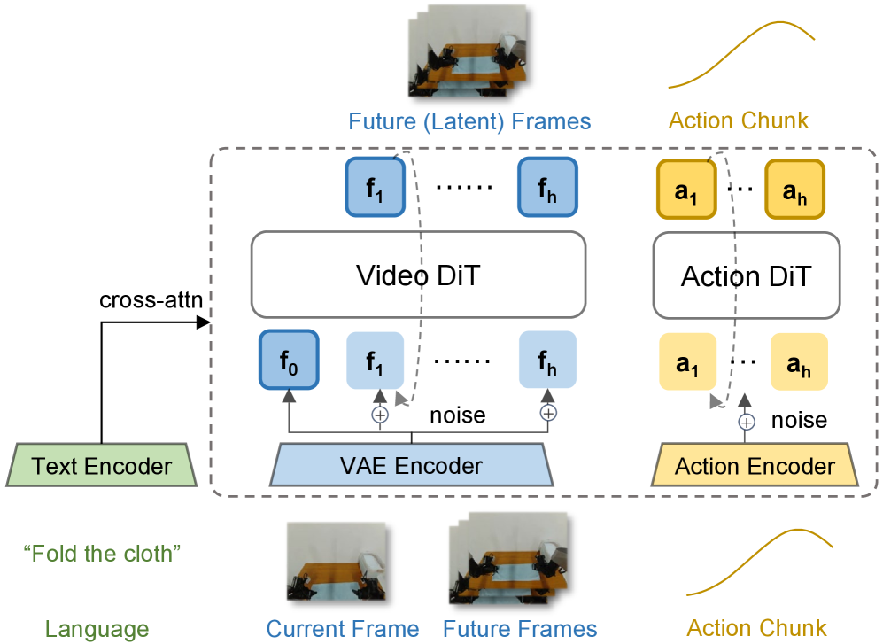
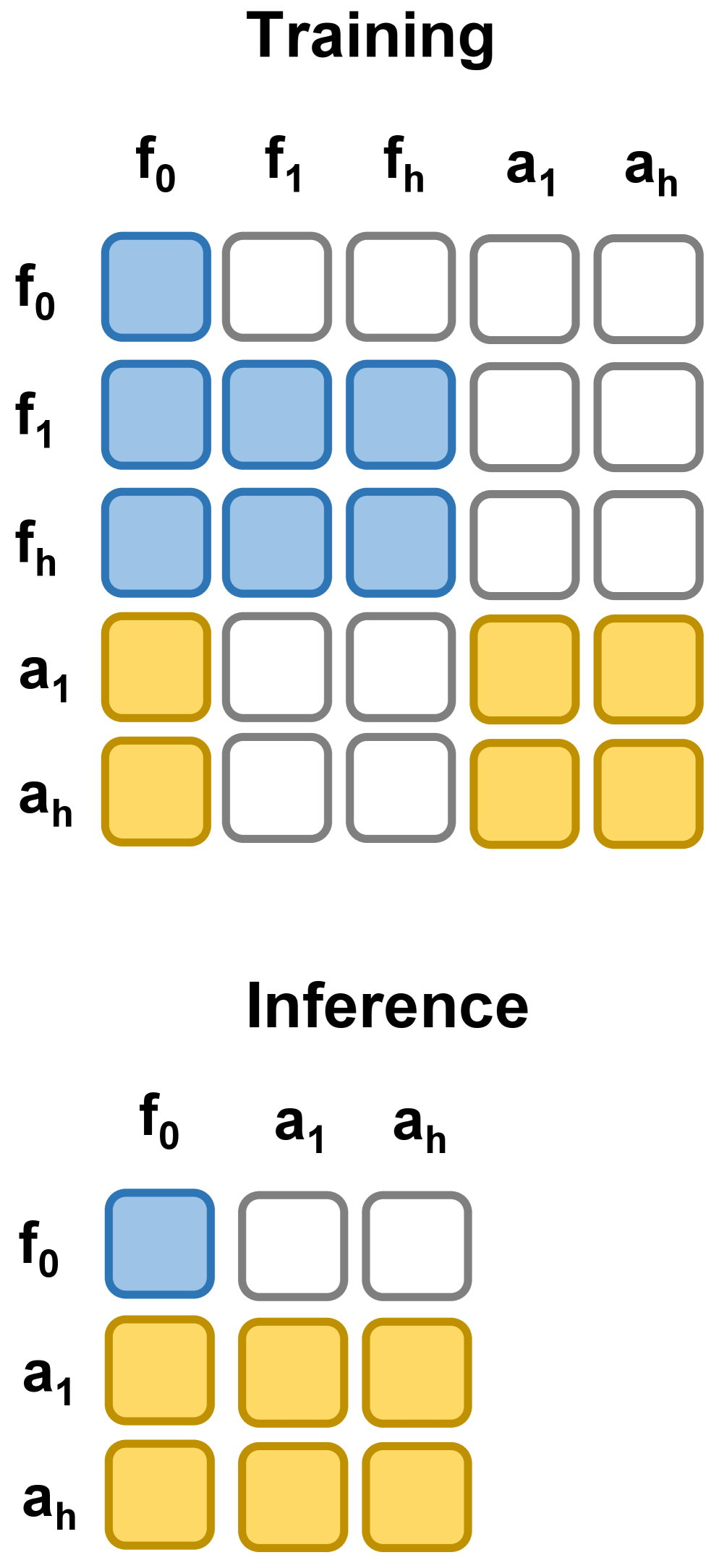
Figure 2 of the paper makes the MoT layout and the train/inference mask split explicit. Panel (a) shows how video tokens and action tokens flow through their respective DiT experts while sharing a single attention pool; panel (b) shows the masks — at training all video tokens are noised so the video loss is alive, while at inference the first observation frame stays clean and no future video is denoised.

论文 Figure 2 把 MoT 布局和训练 / 推理掩码的差异画得很清楚。(a) 展示视频 token 与动作 token 各自走自己的 DiT 专家、但共享同一个 attention 池；(b) 展示掩码——训练时所有视频 token 都被加噪，视频损失保持有效；推理时只有第一帧观测保持干净，且不对任何未来视频做去噪。

At test time, Fast-WAM does not denoise any future video tokens. It keeps only the clean latent tokens of the first observation frame, runs them through the video DiT once (no iterative denoising of \(z_{1:T}\)), and lets the action expert denoise the action chunk with 10 steps and CFG scale 1.0. The video pathway provides representations; the action pathway provides actions; nothing else is materialized.

This is the key efficiency win. On real-world towel folding:

The 4.3× latency reduction is the headline; the 10% success without video co-training is what justifies keeping it during training.

测试时，Fast-WAM 不对任何未来视频 token 去噪。它只保留首帧观测的干净潜 token，让它过一次视频 DiT（不对 \(z_{1:T}\) 做迭代去噪），并让动作专家以 10 步、CFG 系数 1.0 去噪动作块。视频通路提供表示；动作通路输出动作；其余一概不实例化。

这是核心效率收益。在真机叠毛巾任务上：

4.3× 延迟降低是主要卖点；不做视频联合训练时只有 10% 的成功率，正是保留视频联合训练的理由。

The clean experimental design is what makes Fast-WAM’s claim land. Three controlled variants:

• Fast-WAM — video co-training during training, no test-time imagination.
• Fast-WAM-Joint — joint denoising of video and actions at both train and test.
• Fast-WAM-IDM — generate video first, then action via inverse-dynamics model.
• No video co-train — pure action expert, no \(\mathcal{L}_{\text{vid}}\) at all.

Results:

The gap between Fast-WAM and the imagine-then-execute variants (Joint, IDM) is within 1.2% — i.e., test-time imagination is essentially free to skip. The gap between Fast-WAM and the no-video-co-train baseline is 8.0% on RoboTwin and 4.1% on LIBERO. Conclusion: video prediction’s value is in the gradient, not in the rendered frames.

For comparison, LingBot-VA (a model with embodied pretraining) hits 92.2% on RoboTwin and 98.5% on LIBERO. Fast-WAM lands within ~1% of that without any embodied pretraining at all.

Fast-WAM 的论点之所以站得住，靠的是干净的实验设计。三个受控变体：

• Fast-WAM — 训练时视频联合训练，测试时不做想象。
• Fast-WAM-Joint — 训练和测试时都对视频和动作联合去噪。
• Fast-WAM-IDM — 先生成视频，再通过逆动力学模型出动作。
• No video co-train — 纯动作专家，完全没有 \(\mathcal{L}_{\text{vid}}\)。

结果：

Fast-WAM 与 imagine-then-execute 变体（Joint、IDM）的差距在 1.2% 以内——也就是说，测试时的想象基本可以白扔。Fast-WAM 与不做视频联合训练的差距在 RoboTwin 上是 8.0%，在 LIBERO 上是 4.1%。结论：视频预测的价值在梯度里，而不在渲染出来的帧里。

作为对照，LingBot-VA（有具身预训练）在 RoboTwin 上 92.2%、LIBERO 上 98.5%。Fast-WAM 不做任何具身预训练，就落在 ~1% 以内。

With both architectures on the table, two side-by-side comparisons are worth pulling out — first a mechanical one (where the KV cache lives, and why one design is 4× faster), then a philosophical one (the two stances on whether the world model should keep running at deployment).

两个架构都摆出来之后，有两个对比值得单独拎出来：先讲一个机械层面的（KV cache 落在哪里、为什么一个设计快 4×），再讲一个理念层面的（两种立场——部署时世界模型到底要不要继续运行）。

With both architectures on the table, one comparison is worth pulling out before the synthesis: do either of these systems use KV cache sharing at inference, and where does it help? Neither paper names it as a headline optimization, but the two architectures admit it to very different degrees, and the difference is most of the reason Fast-WAM is so much faster.

The trick is: compute keys and values once on tokens that don’t change, then reuse them across many forward passes where something else changes. In autoregressive LLMs the “something else” is the next decoded token, and the cache covers the prefix. In diffusion DiTs the “something else” is the noised target tokens at each denoising step, and the cache covers any clean (unnoised) conditioning tokens — which, by definition, are identical at step \(\tau\) and step \(\tau-1\).

Cosmos Policy. All 11 latent slots go through one bidirectional DiT. At inference, some slots are clean conditioning (current state, language) and others are noised (action, optionally future). Across the 5 denoising steps the noised slots evolve but the clean slots don’t, so their K/V can be cached after the first step and reused. This is a standard inference optimization for any conditional diffusion DiT — the paper doesn’t market it, but the architecture admits it. In planning mode the saving is larger: phase 1 generates the imagined future frames, and in phase 2 those frames become clean conditioning, so phase 1’s full K/V can be carried into phase 2 and only the action slots need fresh computation.

Fast-WAM is the more striking case, and the cache opportunity is in fact what gives the paper its 4× latency win. The Mixture-of-Transformer design makes the entire video branch a one-shot conditioning forward pass at inference — the 5B video DiT runs once on the clean first observation frame and produces no future video at all. Only the 1B action expert iterates (10 denoising steps, CFG = 1.0). Because the shared attention pools Q/K/V from both branches, the video branch’s K/V is what the action expert reads at every step; computing it once and reusing it across all 10 action steps is exactly KV cache sharing applied at the expert boundary rather than at the step boundary. This is the structural reason Fast-WAM beats imagine-then-execute baselines on latency: not faster denoising, but no future denoising at all — the video branch becomes a fixed key/value bank that the action expert queries.

So the high-level contrast is:

• Cosmos’s KV cache lives inside one backbone — clean slots vs noised slots, same DiT, across denoising steps.
• Fast-WAM’s KV cache lives across two backbones — video expert produces, action expert consumes, all 10 action denoising steps reuse the same cache.

Both are special cases of the same underlying observation: clean conditioning is constant across denoising steps, so you should only pay for its K/V once.

A common follow-up: is the video DiT’s K/V also fed into the action DiT during training? In an information-flow sense yes, in a cache sense no. At every training step the video and action branches run together in a single forward pass, and the shared attention freshly pools both branches’ Q/K/V — so the action branch does read the video branch’s K/V, exactly the same way it does at inference. But there is no cache to speak of, because nothing is being reused: each training step sees a different example and a different sampled noise level \(\tau\), the video tokens are noisy (not clean) at training time, and there is no second forward pass that could read a stored cache. The KV cache trick is unique to inference because two conditions only line up there: the video tokens become clean (one shot, no denoising loop) and the action branch iterates over that same fixed video state for 10 steps. At training, neither condition holds — the video state changes every step and there’s only one pass per step — so caching saves nothing and would in fact be wrong (the cache from step \(n\) would be stale by step \(n+1\) because the video tokens have been re-noised at a different level).

The figure below steps through both flows side by side. Hit next (or play) to advance: Cosmos’s clean state slots fill the cache once and are read across 5 denoising steps; Fast-WAM’s video DiT runs once and feeds the action expert across 10 denoising steps.

两个架构都摆出来之后，在做综合之前，有一个对比值得单独拎出来讲：这两个系统是否使用 KV cache sharing 来加速推理？它在哪里发挥作用？两篇论文都没把它写成主打优化，但两边的架构在不同程度上支持这件事，而且这个差异基本就是 Fast-WAM 推理快这么多的主要原因。

这个技巧是：在那些不会变的 token 上把 K/V 算一次，然后让它们被多次前向传播复用——前向之间变的是别的东西。在自回归 LLM 里，变的是下一个被解码的 token，cache 覆盖前缀。在扩散 DiT 里，变的是每一步被加噪的目标 token，cache 覆盖任何干净（未加噪）的条件 token——按定义，第 \(\tau\) 步和第 \(\tau-1\) 步上它们一模一样。

Cosmos Policy。 全部 11 个潜槽都送进同一个双向 DiT。推理时，部分槽是干净条件（当前状态、语言），其他槽是被加噪的目标（动作、可选的未来）。5 个去噪步之间，被加噪的槽在变化，干净的槽不变，因此它们的 K/V 在第一步之后可以被缓存复用。这是任何条件扩散 DiT 都能用的标准优化——论文不会拿它做卖点，但架构允许这么做。规划模式下省得更多：第 1 阶段生成想象的未来帧，进入第 2 阶段时这些帧变成干净条件，所以第 1 阶段的全部 K/V 都可以带入第 2 阶段，只有动作槽需要重新计算。

Fast-WAM 是更有意思的情形——并且这个 cache 机会其实就是 Fast-WAM 4× 延迟收益的来源。它的 Mixture-of-Transformer 设计把整个视频分支变成了推理时的一次性条件前向——5B 的视频 DiT 在干净的首帧观测上跑一次，根本不生成任何未来视频。迭代去噪的只有 1B 的动作专家（10 步，CFG = 1.0）。由于共享 attention 把两个分支的 Q/K/V 池化到一起，动作专家在每一步都要读视频分支的 K/V；把它算一次然后在 10 步里复用，恰好是把 KV cache sharing 施加在专家边界上，而不是步边界上。这就是 Fast-WAM 在延迟上压过 imagine-then-execute 基线的结构原因：不是去噪更快，而是根本不再做未来去噪——视频分支变成一个固定的 K/V 仓库，动作专家来查询。

所以高层对比是：

• Cosmos 的 KV cache 发生在一个主干内部——干净槽 vs 加噪槽，同一个 DiT，跨多个去噪步复用。
• Fast-WAM 的 KV cache 跨越两个主干——视频专家产出，动作专家消费，10 个动作去噪步全部复用同一份 cache。

两者都是同一个底层观察的特例：干净条件在去噪步之间不变，因此你应该只为它的 K/V 付一次代价。

一个常见的追问：训练时视频 DiT 的 K/V 是否也喂给了 action DiT？ 从信息流的角度——是；从 cache 的角度——不是。每个训练 step，视频分支和动作分支在同一次前向里一起跑，共享 attention 现场把两边的 Q/K/V 池化在一起——所以 action 分支确实读到视频分支的 K/V，和推理时一模一样。但这里没有 cache 可言，因为没有任何东西在被复用：每个训练 step 看到不同的样本、不同的采样噪声水平 \(\tau\)，训练时视频 token 是带噪的（不是干净的），并且没有第二次前向可以读一份保存下来的 cache。KV cache 这个 trick 只有在推理时才成立，因为两个条件只有在那里同时满足：视频 token 变成干净的（一次性、没有去噪循环），而 action 分支在那个固定视频状态上迭代 10 步。训练时这两个条件都不成立——视频状态每步都在变、每步只有一次前向——所以缓存什么都省不下，而且本来就错（第 \(n\) 步的 cache 到第 \(n+1\) 步就过期了，因为视频 token 已经被重新加噪到另一个噪声水平上）。

下图把两条 cache 流并排逐步演示。点击 next（或 play）来推进：Cosmos 的干净状态槽把 cache 填一次然后跨 5 步去噪反复读；Fast-WAM 的视频 DiT 跑一次，K/V 给动作专家跨 10 个去噪步读。

The two papers disagree about how much of the world model should run at deployment, but they agree on the underlying mechanism: the world prediction objective is what shapes useful representations.

Cosmos Policy bets that, with enough compute budget, running the world model at test time still pays off — the +12.5 pts on hard ALOHA tasks comes from the planning loop. Fast-WAM bets that for most tasks, the world model has already done its job by the time training ends, and pixel-space rollout at deployment is just expensive denoising.

The synthesis is probably: keep the video co-training loss everywhere, but make the inference-time pixel rollout optional and adaptive — cheap direct decoding when the action is obvious, planning when it isn’t. Neither paper closes that loop yet, but together they sketch the design space.

两篇工作在”部署时多大比例的世界模型该运行”上分歧很大，但它们对底层机制的判断一致：塑造有用表示的，是世界预测目标本身。

Cosmos Policy 押注：算力够大时，测试时真的去跑世界模型仍然划算——ALOHA 难任务上的 +12.5 分就来自规划循环。Fast-WAM 押注：对大部分任务而言，世界模型在训练结束时就已经把活儿干完了，部署时的像素空间 rollout 不过是昂贵的去噪。

合理的综合大概是：到处保留视频联合训练损失，但把推理时的像素 rollout 改成可选且自适应——动作显然时直接解码，否则做规划。这两篇都没有完全闭环，但合起来勾勒出了设计空间。